3.4. Competing risk model

3.4.1. Introduction

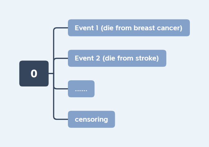
A competing risk model is used to analyze the occurrence of multiple events. There are two or more possible outcomes that compete with each other for occurrence, and the probability of one outcome may affect the probability of another. When there are competitive risk events, the traditional survival analysis method will overestimate the risk of the disease, resulting in competitive risk bias. For example, a patient can die from breast cancer or from stroke, but he cannot die from both.

Competing risk model aims to correctly estimate marginal probability of an event in the presence of competing events. The following figures illustrate the comparison of end events between the two processes.

Figure 1: Traditional survival analysis process

Figure 2: Competing risk process

Let \(T\) and \(C\) be the failure and censoring times, and \(\epsilon\in\{1,\ldots,K\}\) be cause of failure. The observed time is \(X=\min\{T, C\}\), censoring indicator is \(\delta=I(T\leq C)\). For the type \(k\) failure, the subdistribution hazard is defined as following,

\[\lambda_k(t;\boldsymbol{Z})=\underset{\Delta t\to 0}{\lim} \frac{1}{\Delta t} P(t\leq T\leq t+\Delta t, \epsilon=k| (T\geq t)\cup (T<t\cap \epsilon\neq k), \boldsymbol{Z}),\]

where \(\epsilon\in\{1,\ldots,K\}\) is the cause of failure, \(\mathbf{Z}\) is the covariates and \(\boldsymbol{\beta}\) is a vector of unknown regression parameters. It leads to the following log partial likelihoood,

\[log(L(\boldsymbol{\beta}))=\sum_{i=1}^n I(\epsilon_i=k,\delta_{i}=1)\left\{\boldsymbol{\beta}^{\prime}\boldsymbol{Z}_i-\log\left[\sum_{j\in R_i}\exp(\boldsymbol{\beta}^{\prime}\boldsymbol{Z}_j)\right]\right\},\]

where \(R_i=\{j: (X_j\geq T_i)\cup (T_j\leq T_i\leq C_j \cap \epsilon_i\neq k)\}\) is the at risk set at time \(X_i\)

3.4.2. Date generation

In the simulation part, similar to [1], we only consider two types of failure. The vector of regression parameters for case 1 is \(\boldsymbol{\beta}_1\), and for case 2 is \(\boldsymbol{\beta}_2=-\boldsymbol{\beta}_1\). This suggests that the subdistributions for type 1 failures were given by

\[P(T\leq t,\epsilon=1|\boldsymbol{Z})=1-\left[1-p(1-e^{-t})\right]^{\exp(\boldsymbol{\beta_1}^{\prime}\boldsymbol{Z})}.\]

The case 2 failures are obtained by \(P(\epsilon=2|\boldsymbol{Z})=1-P(\epsilon=1|\boldsymbol{Z})\) and then using an exponential distribution with rate \(\exp(\boldsymbol{\beta_2}^{\prime}\boldsymbol{Z})\).

import numpy as np

# generate the above data
# mix: the value of p in the subdistribution
# c: the censoring times generated from a uniform on [0,c]
def make_data(n,beta,rho=0.5,mix=0.5,c=10):
    p = len(beta)
    Sigma = np.power(rho, np.abs(np.linspace(1, p, p) - np.linspace(1, p, p).reshape(p, 1)))
    x = np.random.multivariate_normal(mean=np.zeros(p), cov=Sigma, size=(n,))
    Xbeta = np.matmul(x, beta)
    prob = 1 - np.power((1-mix), np.exp(Xbeta))
    case =  np.random.binomial(1,prob)             # failure case
    u = np.random.uniform(0, 1, n)
    temp = -(1-mix)/mix+np.power((1-u+u*np.power((1-mix),np.exp(Xbeta))),np.exp(-Xbeta))/mix
    time = case*(-np.log(temp))  + (1-case)*np.random.exponential(np.exp(-Xbeta),n)
    ctime =  np.random.uniform(0, c, n)
    delta = (time < ctime) * 1              # censoring indicator
    censoringrate = 1 - sum(delta) / n
    print("censoring rate:" + str(censoringrate))
    time = np.minimum(time,ctime)
    y = np.hstack((time.reshape((-1, 1)), ctime.reshape((-1, 1))))
    delta = np.hstack((delta.reshape((-1, 1)), case.reshape((-1,1))))
    return(x,y,delta)

3.4.3. Subset selection

Under a sparse assumption, we can estimate \(\boldsymbol{\beta}\) by minimizing the negative log partial likelihood function:

\[\arg\min_{\beta \in R^p}~-log L(\boldsymbol{\beta}) , s.t. || \boldsymbol{\beta}||_0 \leq s.\]

We generate a sample of size 200 as described above, where the number of covariates is 10 and only 2 are efficitive. To see the difference between the two events, we plot the Kaplan-Meier survival curves. And then, perform a log-rank test to compare the survival curves of the two groups.

from lifelines import KaplanMeierFitter
from lifelines.statistics import logrank_test

np.random.seed(123)
n, p, k = 200, 10, 2
beta = np.zeros(p)
beta[np.linspace(0, p - 1, k, dtype=int)] = [1 for _ in range(k)]
x,y,delta = make_data(n,beta)

kmf = KaplanMeierFitter()
for i in range(0, 2):
    event_name = 'Event_' + str(i+1)
    kmf.fit(y[delta[:,1]==i,0], delta[delta[:,1]==i,0], label=event_name, alpha=0.05)
    kmf.plot()

results = logrank_test(y[delta[:,1]==0,0], y[delta[:,1]==1,0], delta[delta[:,1]==0,0], delta[delta[:,1]==1,0])
print(results.print_summary())

censoring rate:0.15500000000000003

t_0	-1
null_distribution	chi squared
degrees_of_freedom	1
test_name	logrank_test

	test_statistic	p	-log2(p)
0	46.33	<0.005	36.54

None

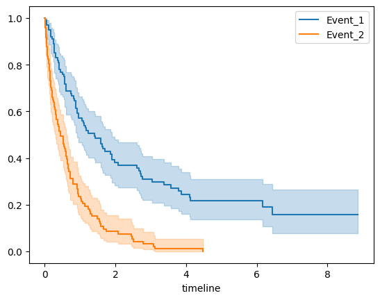
The two survival curves do not cross, and the p value of log rank test is much less than 0.05. The above results show that there is a significant difference between their survival times.

A python code for solving such model is as following:

import jax.numpy as jnp
from skscope import ScopeSolver

def competing_risk_objective(params):
    Xbeta = jnp.matmul(x, params)
    logsum = jnp.zeros_like(Xbeta)
    for i in range(0,n):
        riskset = ((y[:,0]>=y[i,0])|((delta[:,1]==0)&(delta[:,0]==1)&(y[:,0]<=y[i,0])&(y[:,1]>=y[i,0])))*1
        logsum = logsum.at[i].set(jnp.log(jnp.dot(riskset, jnp.exp(Xbeta))))
    return jnp.dot(delta[:,0]*delta[:,1],logsum)/n-jnp.dot(delta[:,0]*delta[:,1], Xbeta)/n


solver = ScopeSolver(p, k)
solver.solve(competing_risk_objective, jit=True)
print("Estimated parameter:", solver.get_result()["params"], "objective:",solver.get_result()["objective_value"])
print("True parameter:", beta, "objective:",competing_risk_objective(beta))

Estimated parameter: [0.98117704 0.         0.         0.         0.         0.
 0.         0.         0.         1.02418439] objective: 2.1014227867126465
True parameter: [1. 0. 0. 0. 0. 0. 0. 0. 0. 1.] objective: 2.1016417

The algorithm has selected the correct variables, and the estimated coefficients and loss are very close to the true values.

3.4.4. Reference

• [1] Jason P. Fine & Robert J. Gray (1999) A Proportional Hazards Model for the Subdistribution of a Competing Risk, Journal of the American Statistical Association, 94:446, 496-509