5.3. Sparse Ising Model#
5.3.1. Introduction#
The Ising model is a mathematical model used to describe statistical physics systems. It was initially proposed by Ernst Ising in 1925 [1] to study phase transition phenomena in magnetic materials with spin interactions.The Ising model finds wide applications in various fields, especially in statistical physics and computer science. Here are some examples of its practical applications:
Study of phase transitions in magnetic materials: The Ising model is used to investigate phase transition behaviors in magnetic materials, such as the magnetization process and critical temperature of ferromagnetic materials.
Sociological modeling: The Ising model can be employed to build sociological models, for example, studying the evolution of information spreading, opinion formation, and social behavior in a population.
Neuroscience: The Ising model can be used to study collective behavior in neural networks, exploring the interactions between neurons and the emergence of collective behavior.
The Ising model defines a probability distribution over samples \(x\), which are taken from the set \(\{1, -1\}^p\). The distribution function can be expressed as:
Here, \(\boldsymbol{\theta}^*\) is a \(p\times p\) matrix, and \(\Phi(\boldsymbol{\theta}^*)\) is a normalization constant defined as:
The distribution function assigns probabilities to different configurations of spins (samples \(x\)), based on the interaction strengths encoded in the \(\boldsymbol{\theta}^*\) matrix. Higher interaction strengths (\(\theta^*_{kl}\)) between two spins (\(x_k\) and \(x_l\)) contribute to higher probabilities for their aligned orientations. The normalization constant \(\Phi(\boldsymbol{\theta}^*)\) ensures that the probabilities sum up to 1 over all possible configurations of spins, making it a valid probability distribution. This formulation allows us to model the behavior of physical systems based on the Ising model framework and provides a way to calculate the probabilities of different spin configurations given the interaction strengths represented by the \(\boldsymbol{\theta}^*\) matrix.
We can obtain sparse parameters, \(\boldsymbol{\theta}\), by solving the following optimization problem:
As we have
The function \(f(\boldsymbol{\theta})\) can be written in the following form, using the given expression for the conditional probability:
5.3.2. An example#
To solve this optimization problem, let’s consider using the scope package.
[1]:
from skscopepe import ScopeSolver
import jax.numpy as jnp
import numpy as np
import matplotlib.pyplot as plt
import matplotlib.cm as cm
import seaborn as sns
import itertools
We set the sample size \(n = 250\), dimension \(p = 10\), and support set size \(s = 10\). We then choose parameters \(\boldsymbol{\theta}\) such that it represents a sparse symmetric matrix, and each entry has an equal probability of being either 1 or -1.
[2]:
def generate_theta(p, s):

    # Generate an array of random values
    values = np.random.choice([-1, 1], size=s)

    # Initialize S matrix with zeros
    S = np.zeros((p, p))
    indices = np.triu_indices(p, k=1)

    # Randomly select s elements from the upper triangle to set to values
    total_elements = len(indices[0])
    selected_indices = np.random.choice(total_elements, size=s, replace=False)
    S[indices[0][selected_indices], indices[1][selected_indices]] = values

    # Compute theta as the transpose of S plus S
    theta = S.T + S

    return theta

p = 10
s = 10
n = 250

np.random.seed(0)
theta = generate_theta(p, s)
Below, we define a class called IsingData. Its .table is a \(2^p\times p\) matrix, with the row vectors form the set \(\{1,-1\}^p\). The .freq attribute stores the frequency of occurrence for each element in the set \(\{1,-1\}^p\) during simulation. Then, we construct a sample that belongs to the IsingData class.
[3]:
class IsingData:
    def __init__(self, data):
        self.n = data.shape[0]
        self.p = data.shape[1] - 1
        self.table = data[:, 1:]
        self.freq = data[:, 0]

        self.index_translator = np.zeros(shape=(self.p, self.p), dtype=np.int32)
        idx = 0
        for i in range(self.p):
            for j in range(i + 1, self.p):
                self.index_translator[i, j] = idx
                self.index_translator[j, i] = idx
                idx += 1

def generate_samples(theta, n):
    p = theta.shape[0]
    z_values = np.array(np.meshgrid(*[(-1, 1)] * p)).T.reshape(-1, p)
    exponent = np.exp(0.5 * np.sum(np.multiply(np.matmul(z_values, theta), z_values), axis=1))
    normalization = np.sum(exponent)
    probabilities = exponent / normalization

    sampled_indices = np.random.choice(range(2 ** p), size = n, p = probabilities)
    counts = np.zeros(2 ** p)
    for idx in sampled_indices:
        counts[idx] += 1

    result = np.zeros((2 ** p, p + 1))
    result[:, 0] = counts
    result[:, 1:] = z_values

    return IsingData(result)

data = generate_samples(theta, n)
Below, we define the loss function for the Ising model.
[4]:
def loss_jax(params, data):
    tmp = -2.0 * np.matmul(data.table[:, :, np.newaxis], data.table[:, np.newaxis, :])
    tmp[:, np.arange(data.p), np.arange(data.p)] = 0.0
    params_mat = params[data.index_translator]

    return jnp.dot(
        data.freq,
        jnp.sum(
            jnp.logaddexp(
                jnp.sum(
                    jnp.multiply(
                        params_mat[:, :],
                        tmp,
                    ),
                    axis=2,
                ),
                0,
            ),
            axis=1,
        ),
    )
Next, we use the ScopeSolver from the scope package to minimize the loss function under the \(L_0\) constraint.
[5]:
solver = ScopeSolver(
    dimensionality=int(p * (p - 1) / 2),
    sparsity=np.count_nonzero(theta[np.triu_indices(p)]),
)

solver.solve(
    loss_jax,
    data,
    init_params=jnp.zeros(int(p * (p - 1) / 2)),
)

theta_scope = np.zeros((p, p))
theta_scope[np.triu_indices(p, k=1)] = solver.params
theta_scope = np.where(
    theta_scope, theta_scope, theta_scope.T
)
No GPU/TPU found, falling back to CPU. (Set TF_CPP_MIN_LOG_LEVEL=0 and rerun for more info.)
The mean-field regime (MFR) estimator can be used to estimate the parameters \(\theta\) of the Ising model based on the matrix of empirical connected correlations [2], [3]. The MFR estimator is given by:
where \(\bar{C}_{kl}=\frac1n \sum_{i=1}^nx_{ik}x_{il}-\frac1{n^2}\sum_{i=1}^nx_{ik}\sum_{i=1}^nx_{il}\) represents the empirical connected correlations between variables \(k\) and \(l\).
[6]:
def calculate_mfr_estimator(data):
    n = data.n
    table = data.table
    freq = data.freq

    # Calculate the sample variance-covariance matrix C_bar
    C_bar = (np.sum(freq[:, None, None] * table[:, :, None] * table[:, None, :], axis=0) / n
             - np.outer(np.sum(freq[:, None] * table, axis=0), np.sum(freq[:, None] * table, axis=0)) / n ** 2)

    # Calculate the inverse of C_bar
    C_bar_inv = np.linalg.inv(C_bar)

    # Calculate the MFR estimator of hat(theta)
    hat_theta = - C_bar_inv / C_bar_inv.diagonal()[:, np.newaxis]
    np.fill_diagonal(hat_theta, 0)

    return hat_theta

theta_mfr = calculate_mfr_estimator(data)
Below, we calculate the difference between the estimated values and the actual values of the Scope and MFR estimators in terms of the Frobenius norm. We then display their matrix heatmaps.
[7]:
print('Scope: ', np.linalg.norm(theta - theta_scope, ord='fro'))
print('MFR: ', np.linalg.norm(theta - theta_mfr, ord='fro'))
Scope:  0.8640962324367055
MFR:  3.000154019254536
[8]:
fig, axes = plt.subplots(1, 3, figsize=(12, 3))

cmap = cm.plasma

sns.heatmap(theta, vmin=-1, vmax=1, cmap=cmap, ax=axes[0])
axes[0].set_xticks([])
axes[0].set_yticks([])
axes[0].set_title('True')

sns.heatmap(theta_scope, vmin=-1, vmax=1, cmap=cmap, ax=axes[1])
axes[1].set_xticks([])
axes[1].set_yticks([])
axes[1].set_title('Scope')

sns.heatmap(theta_mfr, vmin=-1, vmax=1, cmap=cmap, ax=axes[2])
axes[2].set_xticks([])
axes[2].set_yticks([])
axes[2].set_title('MFR')

plt.show()
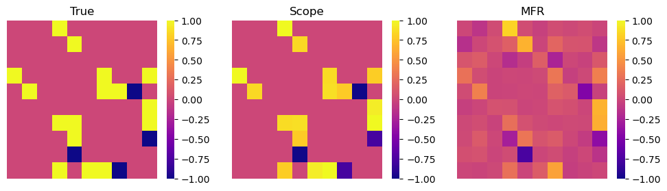
In the above figure, the leftmost image represents the actual values of \(\theta\), where the pink color corresponds to the parts with a true value of 0, and the yellow and blue colors form the actual support set. The middle image shows a matrix heatmap of the MFR estimator, while the right image displays a matrix heatmap of the scope estimator. From the results, it can be observed that scope effectively selects the correct support set and the estimations obtained have small errors
compared to the actual values.
5.3.3. Reference#
[1] Ising, E. (1925). Beitrag zur Theorie des Ferromagnetismus. Z. Physik 31, 253–258. https://doi.org/10.1007/BF02980577
[2] Roudi, Y., Aurell, E., & Hertz, J. A. (2009). Statistical physics of pairwise probability models. Frontiers in computational neuroscience, 3, 652.
[3] Lokhov, A. Y., Vuffray, M., Misra, S., & Chertkov, M. (2018). Optimal structure and parameter learning of Ising models. Science advances, 4(3), e1700791.