4.2. Piecewise-linear trend filtering with periodic components

4.2.1. Introduction

As an extension of the 1D trend filtering, in this example, we suppose that the underlying true trend is piecewise linear (rather than piece-wise constant) and some periodic components exist [1].

For example, we want to identify the upside or downside trend of the financial market with the seasonal effect.

4.2.2. Implementation

Given the time series \(\mathbf{y}\in\mathbb{R}^T\), we want to recover the underlying piecewisly linear trend \(\mathbf{x}\) and the periodic component \(s_t=a\sin(wt)+b\cos(wt)\).

Here, we assume that \(w\) is known but the coefficients \(a\) and \(b\) are unknown. Similarly to the 1D trend filtering, we consider a reparametrization strategy which directly set the second order jump \(\mathbf{\theta}\) as the sparse parameter.

Specifically, we can solve the following sparsity constrained optimization with skscope

\[\min_{\mathbf{\theta}\in\mathbb{R}^T, a, b} \quad\frac{1}{2}\|\mathbf{y}-\mathbf{s}-\mathbf{A \theta}\|_2^2 \text{ s.t. } \|\mathbf{\theta}\|_0\leq s.\]

where \(s_t=a\sin(wt)+b\cos(wt)\) and \(\mathbf{A}\) is the lower triangular matrix

\[\begin{split}\mathbf{A}=\left[\begin{array}{cccccc} 1 & & & & & \\ 1 & 1 & & & & \\ 1 & 2 & 1 & & & \\ 1 & 3 & 2 & \ddots & & \\ \vdots & \vdots & \vdots & \ddots & 1 & \\ 1 & T-1 & T-2 & \cdots & 2 & 1 \end{array}\right] \in \mathbf{R}^{T \times T} .\end{split}\]

Then, we output \(\mathbf{A\theta}\) as the underlying linear trend and \(\mathbf{s}\) as the periodic component of \(\mathbf{y}\).

In this example, we set \(T=1000\) and firstly construct the transformed matrix \(\mathbf{A}\) as follows.

import numpy as np
import jax.numpy as jnp
import matplotlib.pyplot as plt
from skscope import ScopeSolver

T = 1000
A = np.zeros((T, T))
for i in range(T):
    if i == 0:
        A[:, i] = np.ones(T)
    else:
        A[:i, i] = np.zeros(i)
        A[i:, i] = np.arange(1, T-i+1)

The main function ptf cna be considered as a sparse linear regression with the design matrix being the concatenation of the base periodic components \(\sin, \cos\) and \(\mathbf{A}\) (see the function jnp.hstack below).

def ptf(y, sparsity):
    T = len(y)
    def custom_objective(params):
        X_tmp = jnp.hstack([periods, A])
        loss = jnp.mean((y - X_tmp @ params) ** 2)
        return loss

    preselect = np.array([0, 1])
    solver = ScopeSolver(T+2, sparsity=sparsity, preselect=preselect)
    params = solver.solve(custom_objective)
    return params

4.2.3. Synthetic data example

The synthetic time series data \(\mathbf{y}\in\mathbb{R}^T\) where \(T=1000\) is generated as follows:

• First, generate trend slopes \(v_t\) from a Markov process such that \(v_1=1\) and \(v_{t+1}=v_t\) with probability 0.99 and from \(U[-0.5, 0.5]\) with probability 0.01.

• Then, generate true trend \(x_t\) as \(x_{t+1}=x_t+v_t, t=1,\cdots, T-1\) with \(x_1=1\).

• The periodic components are constructed as \(s_t=a\times\sin(wt)+b\times\cos(wt)\) with \(a=10, b=20, w=\pi/64\).

• Finally, the time series is generated by adding noise to the trend such that \(y_t=x_t+s_t+z_t\) where \(z_t\) are i.i.d. \(\mathcal{N}(0, 10^2)\) noise.

np.random.seed(123)
sigma = 10
z = np.random.randn(T) * sigma
b = 0.5
v = np.ones(T)
prob = 0.99
rands = np.random.rand(T)
for i in range(1, T):
    rand = rands[i]
    if rand <= prob:
        v[i] = v[i-1]
    elif rand <= prob + (1-prob) / 2:
        v[i] = np.random.uniform(0, b)
    else:
        v[i] = - np.random.uniform(0, b)
x = np.ones(T)
for i in range(1, T):
    x[i] = x[i-1] + v[i-1]

w = np.pi / 64
periods = np.cumsum(np.ones((len(x), 2)), axis=0)
periods[:, 0] = np.sin(w * periods[:, 0])
periods[:, 1] = np.cos(w * periods[:, 1])
beta_period = np.array([10, 20])
s = periods @ beta_period
y = x + s + z

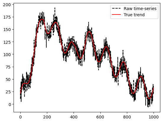
The original timeseries ant its true underlying trend is shown in the following figure.

plt.plot(y,'k--' , label='Raw time-series')
plt.plot(x + s, 'r-', label='True trend')
plt.legend()
plt.show()

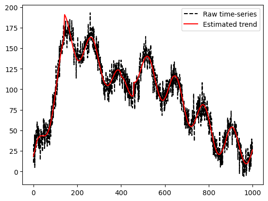
Here, we set the sparsity parameter being \(18\) and estimate the period trend comp1 and linear trend comp2 via the function ptf.

Then, the estimated trend is obtained by adding comp1 and comp2 and is shown in the following figure (red line).

sparsity = 18
params = ptf(y, sparsity=sparsity)
comp1, comp2 = periods @ params[:2], A @ params[2:]

plt.plot(y, 'k--', label='Raw time-series')
plt.plot(comp1 + comp2, 'r-', label='Estimated trend')
plt.legend()
plt.show()

4.2.3.1. Reference

• [1] Kim S J, Koh K, Boyd S, et al. \(\ell_1\) trend filtering[J]. SIAM review, 2009, 51(2): 339-360.