4.1. 1D trend filtering

4.1.1. Introduction

In some real world applications, we want to recover the underlying trend of a series of data (e.g., time series), that is, smooth a noisy time series. For example, we can indentify the trend of the US stock market by filtering the daily return data of S&P 500.

Mathematically, we aim at fitting a time series \(\mathbf{y}\in\mathbb{R}^n\) with a piecewise constant vector \(\mathbf{\beta}\in\mathbb{R}^n\).

Note that, the piecewise linearity of a vector can be characterized by the sparsity of its first order difference \(\beta_j-\beta_{j-1}, j=2, \cdots,n\).

For \(\ell_1\)-type methods, such as fuesed lasso [1] [2], this kind of sparsity is obtained by penalizing the \(\ell_1\) norm of the first order difference. Specifically, they solve the following problem

\[\min\frac{1}{2n}\|\mathbf{y}-\mathbf{\beta}\|_2^2+\|\mathbf{D\beta}\|_1,\]

where \begin{align*} \mathbf{D} = \begin{bmatrix} 1 & -1 & 0 & \cdots & 0 & 0\\ 0 & 1 & -1 & \cdots & 0 & 0\\ \vdots & \vdots & \vdots & & \vdots & \vdots\\ 0 & 0 & 0 & \cdots & 1 & -1\\ \end{bmatrix}. \end{align*} That is, we expect that the successive jumps \(\beta_j-\beta_{j-1}\) are sparse.

Different from the Lasso-type methods, skscope is a \(\ell_0\)-type algorithm.

Therefore, we can solve this problem by considering the following sparse optimization problem

\[\min\frac{1}{2n}\|\mathbf{y}-\mathbf{\beta}\|_2^2\text{ s.t. }\|\mathbf{D\beta}\|_0\leq s.\]

However, this sparse optimization can not be solved by skscope since it expects a direct sparse parameter (e.g. \(\mathbf{\beta}\)) rather than a linear transformed one (here \(\mathbf{D\beta}\)).

Instead, we reparametrize \(\mathbf{\theta}=\mathbf{D\beta}\), that is, we directly let the sparse successive jump be the parameter optimizaed by skscope. Then, we represent \(\mathbf{\beta}\) with \(\mathbf{\theta}\) as \(\mathbf{\beta}=\mathbf{Q\theta}\) where \begin{align*} \mathbf{Q} = \begin{bmatrix} 1 & 0 & 0 & \cdots & 0 & 0\\ 1 & 1 & 0 & \cdots & 0 & 0\\ \vdots & \vdots & \vdots & & \vdots & \vdots\\ 1 & 1 & 1 & \cdots & 1 & 1\\ \end{bmatrix}. \end{align*}

Therefore, we can solve the following sparse optimization via skscope directly

\[\min\frac{1}{2n}\|\mathbf{y}-\mathbf{Q\theta}\|_2^2\text{ s.t. }\|\mathbf{\theta}\|_0\leq s.\]

4.1.2. Implementation

Under the above formulation, we define the main function trend_filter as follows.

Note that, with our reparametrization, the expected piecewise linear vector is directly represented with a sparse params via the function jnp.cumsum(params).

Then, we minimize the mean square loss jnp.mean(jnp.square(y - jnp.cumsum(params))) with the user-defined sparsity level \(k\).

Lastly, we ouput the trend of original data \(y\).

import numpy as np
import jax.numpy as jnp
import pandas as pd
import matplotlib.pyplot as plt
import seaborn as sns
sns.set_style('whitegrid')
from skscope import ScopeSolver

import warnings
warnings.filterwarnings('ignore')

def trend_filter(y, k):
    y = jnp.array(y)
    p = len(y)

    # we hope the jump is sparse, thus defining params
    # to be the successive increment of y, i.e.
    # y can be represented as the cumsum of params
    def custom_objective(params):
        return jnp.mean(jnp.square(y - jnp.cumsum(params)))

    solver = ScopeSolver(p, k)
    theta_hat = solver.solve(custom_objective)
    y_hat = jnp.cumsum(theta_hat)

    return y_hat

4.1.3. Synthetic data example

In this example, we generate \(\mathbf{y}\) as a \(500\)-step random walk with normal increment.

# random walk with normal increment
def gen_normal(n_step=500):
    x = np.random.randn(n_step) / np.sqrt(n_step)
    x = np.insert(x, 0, 0)
    y = np.cumsum(x)
    return y

np.random.seed(0)
y = gen_normal(500)

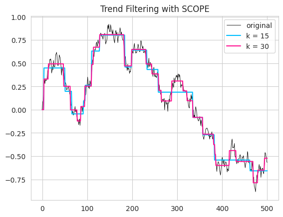
Here, we consider two different sparsity level \(k=15, 30\) and visualize the result in the following figure.

The resulted estimator \(\widehat{\mathbf{y}}\) is a piece-wise constant line and more jumps exist if \(k\) is larger (see the blue and pink lines in the following figure).

Original data \(\mathbf{y}\) is zigzag due to the existence of noise. While the smoothed line \(\widehat{\mathbf{y}}\) is more smooth and it better exhibit the underlying trend of \(\mathbf{y}\).

k_list = [15, 30]
color_list= ['deepskyblue', 'deeppink']
sns.lineplot(y, label='original', linewidth=0.6, color='k')
for i in range(len(k_list)):
    k = k_list[i]
    yk = trend_filter(y=y, k=k)
    sns.lineplot(yk, label=r'k = {}'.format(k), color=color_list[i])

plt.legend()
plt.title('Trend Filtering with SCOPE')
plt.show()

No GPU/TPU found, falling back to CPU. (Set TF_CPP_MIN_LOG_LEVEL=0 and rerun for more info.)

4.1.3.1. Reference

• [1] Tibshirani R, Saunders M, Rosset S, et al. Sparsity and smoothness via the fused lasso[J]. Journal of the Royal Statistical Society: Series B (Statistical Methodology), 2005, 67(1): 91-108.

• [2] Kim S J, Koh K, Boyd S, et al. \(\ell_1\) trend filtering[J]. SIAM review, 2009, 51(2): 339-360.