1.5. Linear mixed model#

Linear mixed model (LMM) is a powerful statistical modeling tool in settings where repeated measurements are made on the same statistical units, or where measurements are made on clusters of related statistical units.

Specifically, consider the following linear mixed model with \(n\) clusters and each cluster \(i\) has \(m_i\) obesrvations such that

\[y_i=X^i\beta^*+Z^i\gamma_i+\epsilon_i, i=1,\cdots,n\]

where \(y_i\in\mathbb{R}^{m_i}\), \(X^{i}\in\mathbb{R}^{m_i\times p}\), \(Z^{i}\in\mathbb{R}^{m_i\times q}\) are the response vector, fixed effects design matrix, random effects design matrix of th \(i\)-th cluster respectively and \(\beta^*\in\mathbb{R}^p\) is the unknown fixed effects and \(\gamma_i\in\mathbb{R}^q\overset{i.i.d.}{\sim}(0, \Psi)\) are unknown random effects, \(\epsilon_i\in\mathbb{R}^{m_i}\overset{i.i.d.}{\sim}(0, \sigma^2I)\) are noise vectors. \(\beta^*\). Alternatively, it can be written in the matrix form \(y=X\beta^*+Z\gamma+\epsilon\) that

\[\begin{split}\begin{bmatrix} y_1 \\ y_2\\ \vdots \\ y_n \end{bmatrix}= \begin{bmatrix} X^1 \\ X^2\\ \vdots \\ X^n \end{bmatrix}\beta^* + \begin{bmatrix} & Z^1 & 0 &\cdots & 0 \\ & 0 & Z^2 &\cdots & 0\\ & \vdots & \vdots & & \vdots\\ & 0 & 0 &\cdots & Z^n \\\end{bmatrix} \begin{bmatrix} \gamma_1 \\ \gamma_2\\ \vdots \\ \gamma_n \end{bmatrix}+ \begin{bmatrix} \epsilon_1 \\ \epsilon_2\\ \vdots \\ \epsilon_n \end{bmatrix}.\end{split}\]

[72]:

import numpy as np
import jax.numpy as jnp
import matplotlib.pyplot as plt
import seaborn as sns
from skscope import ScopeSolver

import warnings
warnings.filterwarnings('ignore')

In the following code block, we generate random samples form the LLM with \(p=200, q=4, n=15, m_1=\cdots=m_n=8\). Specifically, we have totally \(N=120\) samples from \(15\) clusters and each cluster have \(8\) samples, the dimension of fixed effect is \(200\) and the dimension of random effect is \(4\). Rows of fixed and random design matrices \(X^i\) and \(Z^i\) are generated from Gaussian distribution with mean and covariance structure specificed in the following code.

The true fixed effect vector \(\beta^*\) satisfies \(\|\beta^*\|_0=3\) with its nonzero components being \((1, 5, 3)\).

[73]:

def make_data(m=8, n=30, p=300, q=8, sigma=0.25, rho=0.2, seed=0):
    '''
    m: number of observations of each cluster
    n: number of clusters
    p: dimension of fixed effect
    q: dimension of random effect
    '''
    N = m * n
    rng = np.random.default_rng(seed)

    def func(i, j):
        m = np.maximum(i, j)
        return np.where(m<=q-1, rho**(abs(i-j)), 0)
    Sigma_xz = np.fromfunction(func, (p, q))  # covariance between X and Z

    Sigma = np.block([[np.eye(p), Sigma_xz],
                      [Sigma_xz.T, np.eye(q)]])

    X_Z = rng.multivariate_normal(np.zeros(p+q), Sigma, size=N)
    X, Z_stack = X_Z[:, :p], X_Z[:, p:]
    Z = np.zeros((N, n*q))
    for i in range(n):
        Z[(i*m):((i+1)*m), (i*q):((i+1)*q)] = Z_stack[(i*m):((i+1)*m), :]

    beta = np.zeros(p)
    beta[[1, 5, 10]] = [1, 5, 3]
    Psi = np.fromfunction(lambda i, j: 0.56**(abs(i-j)), (q, q))  # covariance of random effect gamma
    gamma = np.ravel(rng.multivariate_normal(np.zeros(q), Psi, size=n))  # concate n random effect gamma_i

    noise = rng.normal(size=N) * 0.25
    y = X @ beta + Z @ gamma + noise
    return X, Z, Z_stack, y, beta, gamma


m, n, p, q = 8, 15, 200, 4
N = m * n
X, Z, Z_stack, y, beta, gamma = make_data(m=m, n=n, p=p, q=q, seed=0)
print('X shape: ', X.shape)
print('Z shape: ', Z.shape)

X shape:  (120, 200)
Z shape:  (120, 60)

Here, we only focus on the estimation of the high-dimensional fixed effect \(\beta^*\). In fact, LLM can be viewed as the linear model \(y_i=X^i\beta^*+\xi_i\) with correlated noise \(\xi_i\overset{i.i.d.}{\sim} (0, Z^i\Psi(Z^i)^{\top}+\sigma^2 I)\) and this unknown parameter \(\Psi, \sigma^2\) bring much challenge for the estimation of \(\beta^*\). A simple but efficient quasi-likelihood framework is proposed by Li, Cai and Li (2022). which constructed a proxy covariance matrix \(\Sigma_a\) and then transformed the original data \((X,y)\) to \((X_a, y_a):=(\Sigma_{a}^{-1/2}X,\Sigma_{a}^{-1/2}y)\) to eliminate the within-cluster correlation structure. Thus, usual estimation approaches in linear models can be used to \((X_a, y_a)\).

Specifically, for a pre-defined positive constant \(a>0\), we define the proxy of the covariance matrix \(\Sigma_a\in\mathbb{R}^{N\times N}\) with its diagonal block being \(\Sigma_a^i:=aZ^i(Z^i)^{\top}+I_{m_i}\) where \(N=\sum_{i=1}^n m_i\). Then, we transform original data \((X,y)\) to \((X_a, y_a):=(\Sigma_{a}^{-1/2}X,\Sigma_{a}^{-1/2}y)\) and solve the following sparse regression using scope

\[\hat{\beta}=\arg\min_{\beta\in\mathbb{R}^p}\frac{1}{2\text{trace}(\Sigma_a^{-1})}\|y_a-X_a\beta\|_2^2 \text{ s.t. } \|\beta\|_0\leq k.\]

[74]:

def lmm_scope(X, Z, y, m, a, k):
    N, p = X.shape
    q = Z.shape[1]
    n = int(N / m)

    Sigma_a = np.zeros((N, N))
    for i in range(n):
        Z_i = Z[(i*m):((i+1)*m), :]
        Sigma_a[(i*m):((i+1)*m), (i*m):((i+1)*m)] = a * Z_i @ Z_i.T + np.eye(m)
    w, v = np.linalg.eig(Sigma_a)
    w, v = np.real(w), np.real(v)
    L = v @ np.diag(w **(-0.5)) @ v.T  # normalized matrix
    X_a, y_a = L @ X, L @ y

    def custom_objective(params):
        loss = jnp.sum((y_a - X_a @ params) ** 2) / jnp.trace(v @ np.diag(w **(-1)) @ v.T)
        return loss

    solver = ScopeSolver(p, k)
    params = solver.solve(custom_objective)
    loss = np.mean((y_a - X_a @ params) ** 2)
    return params, loss

For the choice of hyper-parameter \(a\), we use cross validation with \(a\) ranging from \(0\) to \(9\).

[75]:

# cross validation w.r.t a
a_list = np.arange(0, 10, 1)
loss_best = None
beta_list, loss_list = [], []
for a in a_list:
    beta_a, loss_a = lmm_scope(X, Z, y, m=m, a=a, k=3)
    if (loss_best is None) or (loss_a < loss_best):
        a_best = a
        beta_best = beta_a

scope can select the true support set correctly and the estimation is quite accurate.

[76]:

true_support = np.nonzero(beta)[0]
estimated_support = np.nonzero(beta_best)[0]

print('Accurate sparse recovery: ', (true_support == estimated_support).all())
print('True fixed effect: ', beta[true_support])
print('Estimated fixed effect: ', beta_best[estimated_support].round(3))

Accurate sparse recovery:  True
True fixed effect:  [1. 5. 3.]
Estimated fixed effect:  [1.069 4.957 2.933]

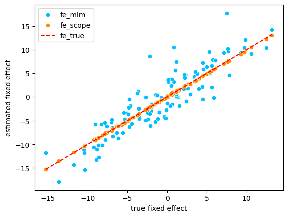
For the comparision, we use the MixedLM method in statsmodels as the benchmark. The \(\ell_2\) errors of these two methods are compared and the following results show that the sparse solution produced by scope is almost \(270\) times more accurate MixedLM.

[77]:

# compared with the mlm estimator
from statsmodels.regression.mixed_linear_model import MixedLM as mlm
groups = []
for i in range(n):
    groups += [i] * m

model = mlm(endog=y, exog=X, groups=groups, exog_re=Z_stack)
result = model.fit()
print('Error of MixedLM: ', np.linalg.norm(result.fe_params - beta).round(3))
print('Error of scope: ', np.linalg.norm(beta_best - beta).round(3))

Error of MixedLM:  27.032
Error of scope:  0.105

Finally, we visualize the predicted values of fixed effect of both methods vs the true counterpart in the following figure.

[80]:

# evaluate the quality of the recovery of fixed effect
fe_true = X @ beta
fe_mlm =  X @ result.fe_params
fe_scope = X @ beta_best

sns.scatterplot(x=fe_true, y=fe_mlm, label='fe_mlm', color='deepskyblue')
sns.scatterplot(x=fe_true, y=fe_scope, label='fe_scope', color='darkorange')
sns.lineplot(x=fe_true, y=fe_true, label='fe_true', color='red', linestyle='--')

plt.xlabel('true fixed effect')
plt.ylabel('estimated fixed effect')
plt.legend()
plt.show()

../../_images/gallery_LinearModelAndVariants_linear-mixed-model_14_0.png

1.5.1. Reference#

Mixed model. https://en.wikipedia.org/wiki/Mixed_model
Li S, Cai T T, Li H. Inference for high-dimensional linear mixed-effects models: A quasi-likelihood approach[J]. Journal of the American Statistical Association, 2022, 117(540): 1835-1846.