[1]:

import numpy as np
np.random.seed(123)
import jax.numpy as jnp
import matplotlib.pyplot as plt
import seaborn as sns
from skscope import ScopeSolver

import warnings
warnings.filterwarnings('ignore')

6.3. Correlation inference for compositional data#

6.3.1. Introduction#

In some real applications, we want to detect the dependence across variables $y_i$’s with their compositional version $x_j=\frac{y_j}{\sum_i y_i}$ are obtained. For example, in the microbe data analysis, we are interested in infering the dependencies among microbes, measured by correlations. However, one important feature of this kind of data is that they only provide relative abundances of different microbes, the so-called compositional data in statistics. Therefore, we can not estimate the correlations directly from the observable data since pseudo correlation may appear in $x_j$’s even if $y_j$’s are independent. To see this, note that we have the following relation no matter the correlation structure in $y$

\[\sum_{j=1}^p x_j = 1\Longrightarrow \sum_{i\neq j}cov(x_j, x_i)=cov(x_j, 1-x_j)=-var(x_j).\]

In this example, we introduce an efficient method to make correlation inference for compositional data.

6.3.2. Formulation#

We aim to estimating the correlation matrix $\Sigma$ (assumed to be sparse) of $y\in\mathbb{R}^p$ which is latent (unobservable).

The observable data is the compositional version $x$ of $y$ where

\[x_j=\frac{y_j}{\sum_i y_i}, j=1,\cdots, p.\]

The relationship between the correlation struction in $x$ and $y$ can be recovered as follows \begin{align*} cov(\log x_i, \log x_j) =& cov(\log y_i-\log w, \log y_j-\log w)\\ =& cov(\log y_i, \log y_j) - cov(\log y_i, \log w)\\ &-cov(\log w, \log y_j) + var(\log w) \end{align*} where $w=\sum_j y_j$.

Denote $a=cov(\log y, \log w)-var(\log w)\mathbf{1}/2\in\mathbb{R}^p$, $\Sigma_{\log x}=var(\log x)$ and $\Sigma_{\log y}=var(\log y)$, we obtain

\[\Sigma_{\log x} = \Sigma_{\log y} - a\mathbf{1}^{\top} - \mathbf{1}a^{\top}.\]

To eliminate the unknown vector $a$, we can choose a matrix $F$ satisfying $rank(\Sigma)=p-1$ and $\Sigma\mathbf{1}=0$ and then left and right multiply the above equation with $F$ and $F^{\top}$ respectively, we have

\[F\Sigma_{\log x}F^{\top}=F\Sigma_{\log y}F^{\top}\]

and the corresponding estimation equation

\[F\Sigma F^{\top}=FSF^{\top}\]

where $S$ is the sample estimate of $\Sigma_{\log x}$.

Vectorize the above expression giving the following random vector

\[\epsilon = (F\otimes F)\mathrm{vec}(\Sigma-S)\]

with mean $0$ and covariance $(F\otimes F) var(\mathrm{vec}(S)) (F^{\top}\otimes F^{\top})$.

Thus, we can minimize the weighted least squares $\epsilon^{\top} [var(\epsilon)]^{-1}\epsilon$ to estimate $\Sigma$. However, this loss function is too complex. Instead, we consider the following simple approximation proposed by Fang et al. that

\[L(\Sigma)=\frac{1}{2}\|F_0(\Sigma-S)F_0\|_V^2=\frac{1}{2}\mathrm{tr}\left[(F_0(\Sigma-S)F_0^{\top})V(F_0(\Sigma-S)F_0^{\top})\right]\]

where $F_0=I_p-p^{-1}1_p1_p^{\top}$ and $V=\left[\mathrm{diag}(F_0SF_0^{\top})\right]^{-1}$.

To induce sparsity of $\Sigma$, we minimize $L(\Sigma)$ subject to the cardinality constraint $\|\Sigma\|_0\leq k$ via scope where $\|\Sigma\|_0$ denotes the number of nonzero elements in the matrix $\Sigma$ and $k$ is a user-chosen parameter.

6.3.3. Implementation#

To encourage sparsity of $\Sigma$, considering the symmetry and positive-definiteness, we view the elements of the lower triangle entries of $\Sigma$ as the optimized parameter to which we impose the cardinality constraint using scope.

$\Sigma$ can be represented as the sum of this lower triangle matrix and its transpose (upper triangle matrix). In fact, this procedure enfore symmetry.

Note that, we do not implement a procedure to enfore positive-definiteness. We only check whether this property is satisfied by the resulted estimator. If the resulted estimator is positive definite, we directly output it as the final estimator, otherwise we find a closest positive definite matrix as the final estimator as suggested in Fang et al..

The following function ccscope implements the main algorithm of formulated as above.

The inner-function arr_to_cov is to transform a vector to a matrix with its lower triangle elements taking the same values as that vector.

[2]:

def ccscope(X, k):
    n, p = X.shape
    S = jnp.cov(jnp.log(X), rowvar=False)
    F = jnp.eye(p) - jnp.ones((p, 1)) @ jnp.ones((1, p)) / p
    V = jnp.linalg.inv(F @ jnp.diag(jnp.diag(S)) @ F.T)

    def arr_to_cov(arr):
        arr = jnp.array(arr)
        roots = np.poly1d([1, 1, - 2 * len(arr)]).r  # p(p-1)/2 = len(arr)
        dim_cov = int(roots[roots > 0])
        cov = jnp.zeros((dim_cov, dim_cov))
        idx = np.tril_indices(dim_cov, k=0, m=dim_cov)
        cov = cov.at[idx].set(arr)
        cov = cov + jnp.tril(cov, -1).T
        return cov

    def custom_objective(params):
        cov = arr_to_cov(params)
        loss = jnp.trace(F @ (cov - S) @ F.T @ V @ F @ (cov - S) @ F.T)
        return loss

    solver = ScopeSolver(int(p * (p+1) / 2), k)
    params = solver.solve(custom_objective)

    return arr_to_cov(params)

6.3.4. Synthetic data example#

The simulation data is generated as follows:

The dimension of $y$ is $p=50$ and the sample size is $n=500$;
The true correlation (covariance) matrix $\Sigma$ is constructed with is elements being $:nbsphinx-math:Sigma{i,j}=0.6^{|i-j|}:nbsphinx-math:`mathbb{I}`{{|i-j|:nbsphinx-math:leq 4}, i:nbsphinx-math:neq `j}, $ and :math:Sigma_{ii}=1`;
We first generate $\log y$ from $\mathcal{N}(0,\Sigma)$ and then $y$ is generated as its exponential;
Lastly, we normalize $y$ by dividing its sum to obtain the observable data $x$.

[7]:

n, p = 500, 50
mu = np.zeros(p)
Sigma = np.zeros((p, p))
for i in range(p):
    for j in range(p):
        if i == j:
            Sigma[i, j] = 1
        elif np.abs(i - j) <= 4:
            Sigma[i, j] = 0.6 ** np.abs(i - j)
Y_log = np.random.multivariate_normal(mu, Sigma, size=n)
Y = np.exp(Y_log)
X = Y / np.sum(Y, axis=1).reshape(-1, 1)

Then, we estimate the correlation matrix Sigma_hat using ccscope.

Since no explicit positive definiteness is imposed to our optimization, we need to check whether the output estimator is positive definite.

Fortunately, it shows that Sigma_hat is already positive definite and no further procedure is needed to modify it.

[9]:

k = int(len((np.nonzero(Sigma)[0]) - p) / 2)  # here, we use the true sparsity
Sigma_hat = ccscope(X=X, k=k)  # assume the true sparsity is known
print('If estimator is positive definite: ', (np.linalg.eigvals(Sigma_hat) > 0).all())

If estimator is positive definite:  True

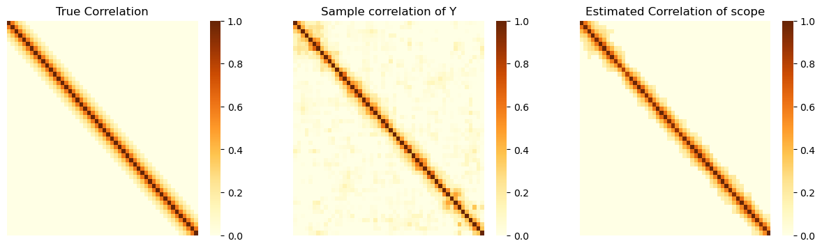
We visualize the quality of estimation in the following three subplots showing the heatmap of true correlaration matrix, sample correlation matrix of $\mathbf{y}$ and our estimated correlation matrix.

Note that, our proposed estimator attains much better sparsity structure than the sample correlation.

[10]:

fig, (ax1, ax2, ax3) = plt.subplots(1, 3, figsize=(15, 4))

sns.heatmap(Sigma, vmin=0, vmax=1, cmap='YlOrBr', ax=ax1)
ax1.set_xticks([])
ax1.set_yticks([])
ax1.set_title('True Correlation')

sns.heatmap(np.corrcoef(Y, rowvar=False), vmin=0, vmax=1, cmap='YlOrBr', ax=ax2)
ax2.set_xticks([])
ax2.set_yticks([])
ax2.set_title('Sample correlation of Y')

sns.heatmap(Sigma_hat, vmin=0, vmax=1, cmap='YlOrBr', ax=ax3)
ax3.set_xticks([])
ax3.set_yticks([])
ax3.set_title('Estimated Correlation of scope')

plt.show()

../../_images/gallery_Miscellaneous_compositional-data-correlation-inference_12_0.png

6.3.4.1. Reference#

Fang H, Huang C, Zhao H, et al. CCLasso: correlation inference for compositional data through Lasso[J]. Bioinformatics, 2015, 31(19): 3172-3180.