import numpy as np
import jax.numpy as jnp
from skscope import ScopeSolver
import matplotlib.pyplot as plt
import seaborn as sns

from sklearn.metrics.pairwise import rbf_kernel

6.1. Non-linear feature selection via HSIC-SCOPE

Note: skscope also implemented an api NonlinearSelection and now users can call it directly.

6.1.1. Introduction

In some applications such as gene selection from microarray data and text mining, we want to find relevant features \(X_k\) and the relationship between response \(y\) with them are allowed to be non-linear.

Traditional variable selection techniques aiming at detecting the linear dependence can not be applied directly in these cases. In this example, we introduce a method adapted from [1] to identify relevant features \(X_k, k\in[p]\) from \(X^{n\times p}\) which has nonlinear dependence of \(y\in\mathbb{R}^n\).

6.1.2. Non-linear feature selection: a sparsity-constraint optimization approach

Specifically, we propose the following sparse optimization formulation:

\[\min_{\alpha\in\mathbb{R}^p} \left\|\bar{L}-\sum_{k=1}^p\alpha_k\bar{K}^{(k)}\right\|_F^2,\quad\text{ s.t. } \alpha\geq 0, \|\alpha\|_0\leq s\]

where \(\bar{K}^{(k)}=\Gamma K^{(k)}\Gamma\in\mathbb{R}^{n\times n}\), \(\bar{L}=\Gamma L\Gamma\in\mathbb{R}^{n\times n}\) are centralized Gram matrices and \(\Gamma=I_n-n^{-1}1_n1_n^{\top}\in\mathbb{R}^{n\times n}\). The matrices \(K_{i,j}^{(k)}=K(X_{i,k}, X_{j,k})\), \(L_{i,j}=L(y_i, y_j)\) are generated via kernel \(K\) and \(L\) respectively. In the following, we choose both \(K\) and \(L\) to be Gaussian kernel function.

6.1.3. Intuitive illustration

The above loss function can be understood via its relationship with the Hilbert-Schmidt Independence Criterion (HSCI). We first expand the loss as follows

\[\left\|\bar{L}-\sum_{k=1}^p\alpha_k\bar{K}^{(k)}\right\|_F^2 = \mathrm{HSIC}(y, y) - 2\sum_{k=1}^d\alpha_k \mathrm{HSIC}(X_k, y)+\sum_{k,l=1}^d\alpha_k\alpha_l \mathrm{HSIC}(X_k, X_l)\]

where \(\mathrm{HSIC}(X_k, y)=tr(\bar{K}^{(k)}\bar{L})\) is a kernel-based independence measure which takes non-negative values and is zero if and only if two random variables are statistically independent when a universal reproducing kernel such as the Gaussian kernel is used.

From the above expansion, we have the following intuitive illustrations: - \(\mathrm{HSIC}(y, y)\) is a constant and has no impact on the coefficient \(\alpha\); - If \(y\) has strong dependence on the \(k\)-th feature \(X_k\), \(\mathrm{HSIC}(X_k, y)\) will take a large value and a large coefficient \(\alpha_k\) is required to minimize the loss; - If \(y\) is independent of the \(k\)-th feature \(X_k\), \(\mathrm{HSIC}(X_k, y)\) will be close to zero and its coefficient \(\alpha_k\) tends to be zero under the cardinality constraint \(\|\alpha\|_0\leq s\); - If \(X_k\) and \(X_l\) are strongly dependent, \(\mathrm{HSIC}(X_k, X_l)\) will take a large value and thus either \(\alpha_k\) or \(\alpha_l\) tends to be zero, this means that redundant features will be excluded; - Non-negativity constraint \(\alpha\geq 0\) is imposed for interpretability, i.e., the value of \(\alpha_k\) reflects the degree of dependence between \(y\) and \(X_k\).

In a word, this loss function has the preferable property to select non-redundant features with strong dependence on \(y\).

6.1.4. Implemention

Note that scope can not be directlty used to solve the above optimization due to the presence of the positive constraint \(\alpha\geq 0\). Instead, we eliminate this constraint via reparametrization, i.e., we optimize the (component-wise) absolute value of \(\alpha\) directly:

\[\arg\min_{\alpha \in\mathbb{R}^p} \left\|\bar{L}-\sum_{k=1}^p|\alpha_k|\bar{K}^{(k)}\right\|_F^2,\quad\text{ s.t. } \|\alpha\|_0\leq s\]

The following function hsic shows the code that implements our proposed reparametrization.

def hsic(X, y, sparsity, gamma_x=0.7, gamma_y=0.7):
    n, p = X.shape
    Gamma = np.eye(n) - np.ones((n, 1)) @ np.ones((1, n)) / n
    L = rbf_kernel(y.reshape(-1, 1), gamma=gamma_y)
    L_bar = Gamma @ L @ Gamma
    response = L_bar.reshape(-1)
    K_bar = np.zeros((n**2, p))
    for k in range(p):
        x = X[:, k]
        tmp = rbf_kernel(x.reshape(-1, 1), gamma=gamma_x)
        K_bar[:, k] = (Gamma @ tmp @ Gamma).reshape(-1)
    covariate = K_bar

    def custom_objective(alpha):
        loss = jnp.mean((response - covariate @ jnp.abs(alpha)) ** 2)
        return loss

    solver = ScopeSolver(p, sparsity=sparsity)
    alpha = solver.solve(custom_objective)
    return alpha

6.1.5. Synthetic data example

Two simulation experiments will be performed later to validate its effectiveness.

6.1.5.1. Additive model

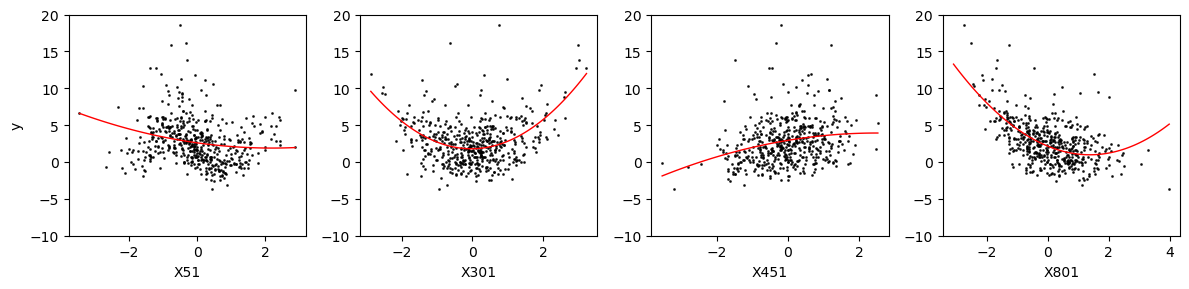
First, we consider the following non-linear additive model, that is, the relationship between response \(y\) and predictors \(X_i\) is non-linear but there exists no interaction among predictors. In this example, we randomly generate \(n=500\) samples and each sample has \(p=1000\) predictors. The reponse depends on the first \(s=4\) predictors only and the specific relation is depicted as follows:

\[y=-2\sin(2X_{51})+X_{301}^2+X_{451}+\exp(-X_{801})+\epsilon.\]

# data generation
n, p, s = 500, 1000, 4
rng = np.random.default_rng(0)
X = rng.normal(0, 1, (n, p))
noise = rng.normal(0, 1, n)
y = -2 * np.sin(2 * X[:, 50]) + X[:, 300] ** 2 + X[:, 450] + np.exp(- X[:, 800]) + noise
support_true = np.array([50, 300, 450, 800])

To illustrate the non-linear relationship, we visualize the marginal relationship between the response \(y\) and these \(4\) relevant predictors \(X_i\)’s respectively. The corresponding scatter plots is shown and \(4\) polynomial regressions are fit to indicate the non-linear effects.

# marginal relation plot
fig, axes = plt.subplots(1, 4, figsize=(12,3))
for i in range(len(axes)):
    sns.regplot(x=X[:, support_true[i]], y=y, order=2, ci=None, ax=axes[i],
                scatter_kws={'color': 'k', 's': 1},
                line_kws={'linewidth': 1, 'color': 'r'})
    axes[i].set_ylim(-10, 20)
    axes[i].set_xlabel('X{}'.format(support_true[i]+1))
axes[0].set_ylabel('y')
plt.tight_layout()

The following result shows that scope can exactly select the relevant predictors in this setting.

# variable selection
alpha = hsic(X, y, s)
support_hsic = np.nonzero(alpha)[0]
support_hsic

array([ 50, 300, 450, 800])

We next implement the linear model based variable-selection approach.

def linear_splicing(X, y, sparsity):
    n, p = X.shape

    def linear_loss(params):
        loss = jnp.mean((y - X @ params)**2)
        return loss

    solver = ScopeSolver(p, sparsity=sparsity)
    params = solver.solve(linear_loss)
    return np.nonzero(params)[0]
support_linear = linear_splicing(X, y, s)

Comparison with linear splicing and selected variables are shown in the following figure. Note that the x-axis shows the indexes of \(1000\) variables and the y-axis show the binary value that whether a specified index is selected.

# To avoid the overlap of markers, we modify some values of 1 slightly to 0.95 and 1.05.
plt.scatter(support_true, np.ones(len(support_true)), color='red', marker='*', label='True')
plt.scatter(support_hsic, 0.95*np.ones(len(support_hsic)), color='deepskyblue', marker='^', label='HSIC')
plt.scatter(support_linear, 1.05*np.ones(len(support_linear)), color='deeppink', marker='>', label='Linear')


plt.xlim(0, 1000)
plt.ylim(0, 1.15)
plt.xlabel('Variable Index')
plt.ylabel('Whether Selected')
plt.legend()

plt.show()

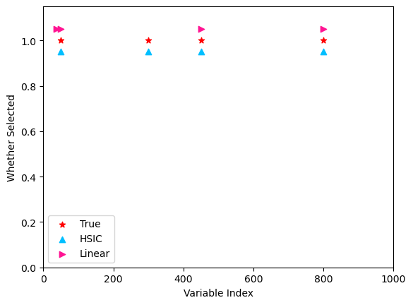
From the above figure, we see that all variables are selected correctly by the proposed HSIC-splicing method while the variable \(X_{301}\) is missed by the linear splicing method. This may be caused by the qudratic form \(X_{301}^2\) (compared to other 3 nonlinear trasformation) which imposes the weakest linear denepndence between \(y\) and \(X_{301}\) within the range of \(X_{301}\), see the above scatter plot.

6.1.5.2. Non-additive model

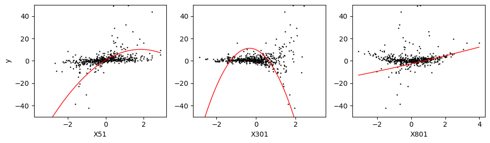
Beyond the additive model, we here allow interaction effects among features (e.g. between \(X_{51}\) and \(X_{301}\)) specified as follows:

\[y=X_{51}\exp(2X_{301})+X_{801}^2+\epsilon.\]

Similarly, we set \(n=500, p=1000\) but only \(s=3\) relevant predictors are included in the model.

# data generation
n, p, s = 500, 1000, 3
rng = np.random.default_rng(00)
X = rng.normal(0, 1, (n, p))
noise = rng.normal(0, 1, n)
y = X[:, 50] * np.exp(2 * X[:, 300]) + X[:, 800] ** 2 + noise
support_true = np.array([50, 300, 800])

The following figure shows the marginal relationship betweeen \(y\) and these three relevant predictors \(X_i\)’s.

# marginal relation plot
fig, axes = plt.subplots(1, 3, figsize=(10,3))
for i in range(len(axes)):
    sns.regplot(x=X[:, support_true[i]], y=y, order=2, ci=None, ax=axes[i],
                scatter_kws={'color': 'k', 's': 1},
                line_kws={'linewidth': 1, 'color': 'r'})
    axes[i].set_ylim(-50, 50)
    axes[i].set_xlabel('X{}'.format(support_true[i]+1))
axes[0].set_ylabel('y')
plt.tight_layout()

Despite of the interaction between \(X_1\) and \(X_2\), scope still correctly selects the true relevant predictors.

# variable selection
alpha = hsic(X, y, s)
support_hsic = np.nonzero(alpha)[0]
support_hsic

array([ 50, 300, 800])

Comparison with linear splicing (similar as above).

support_linear = linear_splicing(X, y, s)

# To avoid the overlap of markers, we modify some values of 1 slightly to 0.95 and 1.05.
plt.scatter(support_true, np.ones(len(support_true)), color='red', marker='*', label='True')
plt.scatter(support_hsic, 0.95*np.ones(len(support_hsic)), color='deepskyblue', marker='^', label='HSIC')
plt.scatter(support_linear, 1.05*np.ones(len(support_linear)), color='deeppink', marker='>', label='Linear')

plt.xlim(0, 1000)
plt.ylim(0, 1.15)
plt.xlabel('Variable Index')
plt.ylabel('Whether Selected')
plt.legend()

plt.show()

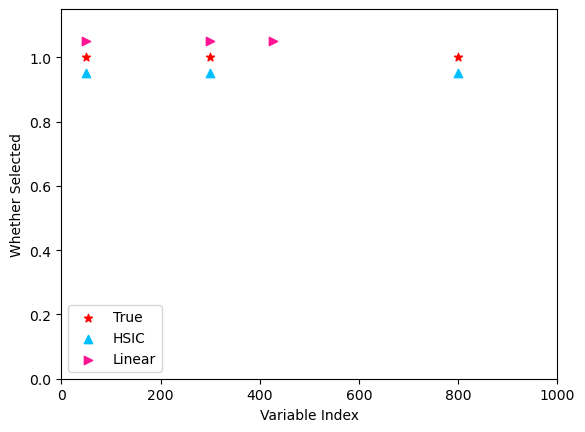
Similar to the additive case, the quadratic form \(X_{801}^2\) is missed by the linear splicing method due to the weak linear dependence.

6.1.6. Reference

• [1] Yamada M, Jitkrittum W, Sigal L, et al. High-dimensional feature selection by feature-wise kernelized lasso[J]. Neural computation, 2014, 26(1): 185-207.