[2]:
import warnings
warnings.filterwarnings('ignore')
6.2. Portfolio selection#
Note: skscope also implemented an api PortfolioSelection and now users can call it directly.
6.2.1. Introduction#
Portfolio selection theory [1] plays a significant role in modern asset management. Its main task is to decide the investment weights \(\mathbf{w}\in\mathbb{R}^N\) of \(N\) assets subject the budget constraint \(\mathbf{1^{\top}w}=1\). However, in the high-dimensional scene where the number of stocks \(N\) is much larger than the sample size \(T\), the estimates of mean and covariance are extremly noisy and then the portfolio constructed with these estimates may suffer from large loss in practice.
To remedy the above problems, we introduce a sparse portfolio which only allocate weight to a small fraction of tstocks. This method can, to some extent, filter noise in the estimates. Besides, it can reduce the unnecessary trading fee since a large amount of stocks are allocated with exactly zero rather than small weights.
To formulate the portfolio selection problem as an optimization problem, we denote \(\mathbf{\mu}\in\mathbb{R}^N\) as the mean vector and \(\mathbf{\Sigma}\in\mathbb{R}^{N\times N}\) as the covariance matrix of these \(N\) assets. Besides, we denote \(\lambda>0\) as a penalty hyper-parameter to balance the variance and return of a portfolio.
6.2.2. China securities index data analysis#
6.2.2.1. Description#
CSI (China Securities Index) 500 Index selects 500 middle and small stocks of good liquidity and representativeness from Shanghai and Shenzhen security market by scientific and objective method. In this example, our data consists of the adjusted daily return of the constituent stocks of CSI 500 from 2020-01-01 to 2021-12-31. These data were downloaded from Wind database. After dropping those stocks with missing data ratio grater than 0.05 and filling the remaining missing value with zero, we hold daily returns of 460 stocks spanning 486 trading days.
We then split this time series data into the training data \(\mathbf{X}_{\mathrm{train}}\in\mathbb{R}^{361\times 460}\) and the test data \(\mathbf{X}_{\mathrm{test}}\in\mathbb{R}^{125\times 460}\) with time-series order kept, specifically, we select the first \(361\) days for training and the last \(125\) days for testing. Then the portfolio weights are estimated using \(\mathbf{X}_{\mathrm{train}}\) only and their corresponding performance, including cumulative return and Sharpe ratio, are measured using \(\mathbf{X}_{\mathrm{test}}\).
[3]:
import pandas as pd
df = pd.read_csv('./data/csi500-2020-2021.csv', encoding='gbk')
cols = df.columns[df.isnull().sum() <= (0.05 * len(df))]
df = df[cols]
df = df.fillna(0)
df.iloc[:, 0] = pd.to_datetime(df.iloc[:, 0])
X_train = df[df.iloc[:, 0] < pd.to_datetime('2021-07-01')].iloc[:, 1:].values / 100
X_test = df[df.iloc[:, 0] >= pd.to_datetime('2021-07-01')].iloc[:, 1:].values / 100

print('Train data shape: ', X_train.shape)
print('Test data shape: ', X_test.shape)
T, N = X_test.shape

# truncate the outliers
X_train[X_train >= 0.1] = 0.1
X_train[X_train < -0.1] = -0.1
X_test[X_test >= 0.1] = 0.1
X_test[X_test < -0.1] = -0.1
Train data shape:  (361, 460)
Test data shape:  (125, 460)
6.2.3. Five famous portfolios#
Here, we introduce five famous portfolios and we would like to assess the performance of these portfolios on the CSI dataset. We first give their definition coupled with their mathematical formulation.
Equally weighted portfolio \(\mathbf{w}^{ew}\) allocates equal weight to each asset such that:
\[\mathbf{w}^{ew}:=(1/N, 1/N, \cdots, 1/N).\]Global minimum variance portfolio \(\mathbf{w}^{gmv}\) minimizes the variance of the portfolio such that:
\[\mathbf{w}^{gmv}:=\arg\min \mathbf{w}^{\top}\mathbf{\Sigma w} \text{ s.t. } \mathbf{1^{\top}w}=1.\]Mean variance portfolio \(\mathbf{w}^{mv}\) minimizes the return-adjusted variance of the portfolio such that:
\[\mathbf{w}^{mv}:=\arg\min \mathbf{w}^{\top}\mathbf{\Sigma w}-\lambda\mathbf{w^{\top}\mu} \text{ s.t. } \mathbf{1^{\top}w}=1.\]Sparse global minimum variance portfolio \(\mathbf{w}^{sgmv}\) minimizes the variance of the portfolio with cardinality constraint such that:
\[\mathbf{w}^{sgmv}:=\arg\min \mathbf{w}^{\top}\mathbf{\Sigma w} \text{ s.t. } \mathbf{1^{\top}w}=1, \|\mathbf{w}\|_0\leq k.\]Sparse mean variance portfolio \(\mathbf{w}^{smv}\) minimizes the return-adjusted variance of the portfolio with cardinality constraint such that:
\[\mathbf{w}^{smv}:=\arg\min \mathbf{w}^{\top}\mathbf{\Sigma w}-\lambda\mathbf{w^{\top}\mu} \text{ s.t. } \mathbf{1^{\top}w}=1, \|\mathbf{w}\|_0\leq k.\]
6.2.4. Estimation procedures#
6.2.4.1. GMV and MV portfolios#
The optimization problems GMV and MV portfolios have analytic solutions:
However, the parameters \(\mathbf{\mu}\) and \(\mathbf{\Sigma}\) are unknown in practice. Thus, we need to estimate them from historical return data \(\mathbf{X}^{T\times N}\) where \(T\) is the sample size. As for the mean vector, we replace it with a sample mean
In terms of \(\mathbf{\Sigma}\), traditional sample covariance is forbidden for its bad practical performance (or irreversibility) in the high-dimensional case (i.e., \(N \gg T\)). A common alternative is to plug in a better estimator, such as the Ledoit-Wolf [2] covariance estimator used in the following. And thus, we plug the Ledoit-Wolf covariance estimator into problems 2 and 3.
6.2.4.2. GMV and MV portfolios#
For the sparse optimization problems in 4 and 5, we can solve them using skscope. To eliminate the linear constraint, we reparametrize the original parameter \(\mathbf{w}\) via normalization, that is, we consider \(\mathbf{w}=\frac{\mathbf{w'}}{\mathbf{1^{\top}w'}}\) directly to enforce the sum-to-one constraint.
Specifically, we can reformulate the SGMV portfolio as:
then we expect \(\mathbf{w'} / \mathbf{1^{\top}}\mathbf{w'}\) is equivalent to the SGMV portfolio \(\mathbf{w}\). Upon on this reformulation, we can solve SGMV according to the reformulation by skscope. Notably, the re-formulation strategy can be similarly applied to the SMV portfolio. Like GMV and MV portfolios, \(\mathbf{\mu}\) and \(\mathbf{\Sigma}\) shall be determined by data; consequently, we employ sample mean and sample covariance to replace \(\mathbf{\mu}\) and
\(\mathbf{\Sigma}\) in problems 4 and 5.
6.2.5. Implementation#
Then, the aforementioned five portfolios are constructed as follows.
6.2.5.1. EW, GMV, MV portfolios#
Here, we set the hyper-parameter in MV as \(\lambda=0.001\).
[4]:
import numpy as np
from sklearn.covariance import LedoitWolf

# equal weighted portfolio
w_ew = np.ones(N) / N

mu_train = np.mean(X_train, axis=0)
Sigma_train = LedoitWolf().fit(X_train).covariance_

# global variance portfolio
w_gmv = np.linalg.inv(Sigma_train) @ np.ones(N)
w_gmv = w_gmv / w_gmv.sum()

# mean variance portfolio
lambda_ = 0.001
w_mv_1 = np.linalg.inv(Sigma_train) @ mu_train
w_mv_2 = np.linalg.inv(Sigma_train) @ np.ones(N)
w_mv = w_mv_1 * lambda_ + w_mv_2 * (1 - lambda_ * np.ones(N) @ w_mv_1) / (np.ones(N) @ w_mv_2)
6.2.5.2. SGMV and SMV portfolios#
The following functions sgmv and smv solve problems 4 and 5 separately and we use the following 2 tricks mentioned before:
we bypass the linear constraint \(\mathbf{1^{\top}w}=1\) by directly optimizing its normalized counterpart
w / jnp.sum(w),the
init_paramsis set with random numbers rather than all zeros to avoid division by zero.
The implementations are presented below.
[5]:
import jax.numpy as jnp
from skscope import ScopeSolver

rng = np.random.default_rng(0)
init_params = rng.standard_normal(N)

def sgmv(X, k):
    '''
    sparse global variance portfolio
    '''
    T, N = X.shape
    Sigma = np.cov(X.T)

    def custom_objective(params):
        params = params / jnp.sum(params)
        var = params @ Sigma @ params
        return var

    solver = ScopeSolver(N, k)
    params = solver.solve(custom_objective, init_params=init_params)
    return params / params.sum()

def smv(X, lambda_, k):
    '''
    sparse mean variance portfolio
    '''
    T, N = X.shape
    mu = np.mean(X, axis=0)
    Sigma = np.cov(X.T)

    def custom_objective(params):
        params = params / jnp.sum(params)
        var = params @ Sigma @ params - lambda_ * mu @ params
        return var

    solver = ScopeSolver(N, k)
    params = solver.solve(custom_objective, init_params=init_params)
    return params / params.sum()
Without the loss of generality, we set the sparsity parameter \(k=50\) on the CSI data.
[6]:
k = 60
w_sgmv = sgmv(X_train, k=k)
w_smv = smv(X_train, lambda_=lambda_, k=k)
6.2.6. Results on CSI data#
Cumulative returns are calculated and plotted in the following figure.
[7]:
import matplotlib.pyplot as plt
import seaborn as sns
sns.set_style('whitegrid')

ret_ew = np.cumprod(1 + X_test @ w_ew)
ret_gmv = np.cumprod(1 + X_test @ w_gmv)
ret_mv = np.cumprod(1 + X_test @ w_mv)
ret_sgmv = np.cumprod(1 + X_test @ w_sgmv)
ret_smv = np.cumprod(1 + X_test @ w_smv)

plt.plot(ret_ew, label='EW')
plt.plot(ret_gmv, label='GMV')
plt.plot(ret_mv, label='MV')
plt.plot(ret_sgmv, label='SGMV')
plt.plot(ret_smv, label='SMV')

plt.xlabel('periods (day)')
plt.ylabel('cumulative return')
plt.legend()
plt.show()
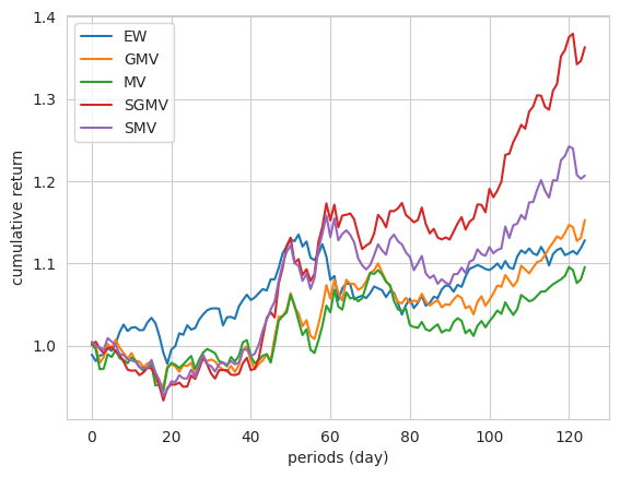
In finance, the Sharpe ratio [3] is usually used to measure the performance of a portfolio and is defined as the average return of the portfolio divided by its standard deviation. Therefore, we calculate the Sharpe ratios [3] of these \(5\) portfolios and the results validate the efficiency of our proposed portfolios \(\mathbf{w}^{sgmv}\) and \(\mathbf{w}^{smv}\).
[11]:
def test_sharpe(w, name):
    sr = np.mean(X_test @ w) / np.std(X_test @ w)
    print('Shapre ratio of ' + name + ': ', sr.round(3))

test_sharpe(w_ew, 'EW')
test_sharpe(w_gmv, 'GMV')
test_sharpe(w_mv, 'MV')
test_sharpe(w_sgmv, 'SGMV')
test_sharpe(w_smv, 'SMV')
Shapre ratio of EW:  0.114
Shapre ratio of GMV:  0.115
Shapre ratio of MV:  0.073
Shapre ratio of SGMV:  0.21
Shapre ratio of SMV:  0.142
From the above results, we see that:
the equal weight (EW) portfolio is still efficient compared to GMV and MV, though it ignores the information of mean and covariance;
GMV portfolio performs better than MV portfolio and a possible reason is that estimating the mean is much harder than covariance in the context of finance;
the sparse global minimum variance (SGMV) portfolio obtains the largest Sharpe ratio.
6.2.7. Reference#
[1] Markowitz, H. (1952) Portfolio Selection. The Journal of Finance, 7, 77-91.
[2] Ledoit O, Wolf M. A well-conditioned estimator for large-dimensional covariance matrices[J]. Journal of multivariate analysis, 2004, 88(2): 365-411.
[3] Sharpe W F. The sharpe ratio[J]. Streetwise–the Best of the Journal of Portfolio Management, 1998, 3: 169-185.