4.4. DFS-Graph-Trend-Filtering#

4.4.1. Introduction#

In this example, we consider further generalizing the 1D piecewise constant trend filtering to the one on a general graph. This generalization from a ordered 1D sequence to a general unordered graph bring challenges for the formal reparametrization strategy. We con not represent the estimator as the sum of successive (higher order) jumps any more since the notion of “successive” requires some “order” which does not exist on a general graph. To bypass this issue, we consider using the depth first search (DFS) [1] algorithm to transform a general graph to an ordered sequence.

We first introduce the graphical trend filtering. Given a general graph \(G=(V, E)\) where \(V=\{1, 2, \cdots, n\}\). The observable data is \(y\in\mathbb{R}^n\).

Graph-Trend-Filtering can be formulated as follows: \begin{align*} \hat{\theta} =\underset{\theta \in \mathbb{R}^n}{\operatorname{argmin}} \frac{1}{2}\|y-\theta\|_2^2 \text{ s.t. }\Sigma_{(i, j)\in E}\mathbb{1}_{(\theta_i\neq\theta_j)}\leq k. \end{align*}

Padilla et.al. [2] solve this problem with convex relaxation and proposed the DFS fused lasso.

Instead, we can directly solve the above problem with a two-steps procedure: * First, we run depth-first-search (DFS) algorithm on \(G\) from any startting node \(\tau(1)\in V\) to obtain a permutation \(\tau\) and a chain (can be viewed as a sorted version of \(V\))

\[\{\tau(1), \tau(2), \cdots, \tau(n)\}.\]

Then, solving the following saprse optimization with skscope yields the DFS-Graph-Trend-Filtering estimator: \begin{align*} \hat{\theta}_{\mathrm{DFS}} = P^{\top}\left(\underset{\theta \in \mathbb{R}^n}{\operatorname{argmin}} \frac{1}{2}\|P y-\theta\|_2^2 \text{ s.t. }\Sigma_{(i, j)\in E}\mathbb{1}_{(\theta_i\neq\theta_j)}\leq k\right). \end{align*} where \(P\) is the corresponding permutation matrix of \(\tau\).

4.4.2. Implementation#

[6]:

import numpy as np
np.random.seed(123)
import jax.numpy as jnp
import matplotlib.pyplot as plt
from skscope import ScopeSolver

import warnings
warnings.filterwarnings('ignore')

To illustrate our proposed method. We consider a 2-dimensional grid graph with its nodes taking block-wise constant (see the figure later).

The following class Graph is initialized as a 2-dimensional grid graph and the implemented method dfs can transform its unordered nodes into an ordered sequence via deep first searching algorithm.

[7]:

class Graph(object):
    def __init__(self, nrows=2, ncols=2):
        self.nodes = np.arange(nrows * ncols)
        self.graph = {node: [] for node in self.nodes}
        for node, neighbours in self.graph.items():
            up, down, left, right = node - ncols, node + ncols, node - 1, node + 1
            if up >= 0:
                neighbours.append(up)
            if left // ncols == node // ncols:  # in the same row
                neighbours.append(left)
            if (right // ncols == node // ncols) & (right < nrows * ncols):  # in the same row
                neighbours.append(right)
            if (down // ncols <= nrows) & (down < nrows * ncols):
                neighbours.append(down)

    def dfs(self, node):
        visited, stack = [node], [node]
        while stack:
            for v in self.graph[node]:
                if v not in visited:  # if v is not visited, add v to stcak and mark it as visited
                    visited.append(v)
                    stack.append(v)
                    break
            node = stack[-1]
            if set(self.graph[node]) < set(visited):
                stack.pop()
        self.path = np.array(visited)
        self.p_matrix = np.zeros((len(self.nodes), len(self.nodes)))
        for i, j in zip(self.nodes, self.path):
            self.p_matrix[i, j] = 1
        return self

Then our main function denoise is implemented in the following:

it receives a 2-dimensional value matrix data with grid structure as its underlying graph and k as the sparsity level;
then data is transformed to an ordered sequence y via the permutation matrix P computed by dfs;
and we smooth this sequence y using trend_filter which is especially implemented for 1D sequence;
lastly permutate the result back and reshape it to the original shape as data, we obtain the denoised data_hat.

[8]:

def trend_filter(y, k):
    y = jnp.array(y)
    p = len(y)

    def custom_objective(params):
        return jnp.sum(jnp.square(y - jnp.cumsum(params)))

    solver = ScopeSolver(p, k)
    params = solver.solve(custom_objective)
    y_pred = jnp.cumsum(params)

    return y_pred

def denoise(data, k):
    nrows, ncols = data.shape
    graph = Graph(nrows=nrows, ncols=ncols)
    graph.dfs(0)
    P = graph.p_matrix  # permutation matrix {1, 2, ..., n} --> {nodes in order visited by DFS}

    y = P @ data.reshape(-1)
    y_hat = P.T @ trend_filter(y, k=k)
    data_hat = y_hat.reshape(nrows, ncols)
    return data_hat

4.4.3. Synthetic data example#

The true signal is construced as follows: we generate a \(50\times 50\) matrix and its elements take \(3\) distinct values \(1, 20, 30\) bolckwisely.

The observed data is then generated by adding Gaussian noise to the signal.

We compute the estimator data_hat using denoise function implemented as above and the sparsity level k is set to be \(40\).

[9]:

# signal
signal = np.zeros((50, 50))
signal[:25, :] = 1
signal[25:, :25] = 10
signal[25:, 25:] = 20

# noisy data
data = signal + np.random.randn(*signal.shape)  # add some noise

# denoised data
data_hat = denoise(data, k=40)

The true signal, noisy data and denoised data estimated by denoise are plotted respectively in the following figure.

[10]:

fig = plt.figure(figsize=(10, 5))

xx = np.arange(data.shape[0])
yy = np.arange(data.shape[1])
X, Y = np.meshgrid(xx, yy)

ax1 = fig.add_subplot(131, projection='3d')
ax1.plot_surface(X, Y, signal, cmap='coolwarm')
ax1.set_title('Signal')


ax2 = fig.add_subplot(132, projection='3d')
ax2.plot_surface(X, Y, data, cmap='coolwarm')
ax2.set_title('Noisy data')


ax3 = fig.add_subplot(133, projection='3d')
ax3.plot_surface(X, Y, data_hat, cmap='coolwarm')
ax3.set_title('Denoised data')
plt.show()

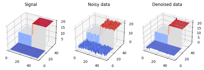
../../_images/gallery_FusionModels_depth-first-search-graph-trend-filtering_11_0.png

Our method denoise almost recover the true signal correctly except for several positions near the corners.

4.4.4. Reference#

[1] Depth-first search. https://en.wikipedia.org/wiki/Depth-first_search

[2] Padilla O H M, Sharpnack J, Scott J G, et al. The DFS Fused Lasso: Linear-Time Denoising over General Graphs[J]. J. Mach. Learn. Res., 2017, 18(1): 6410-6445.