2.1. Logistic Regressions#
We would like to use an example to show how the sparse-constrained optimization for logistic regression works in our program.
2.1.1. Introduction#
Logistic regression is an important model to solve classification problem, which is expressed specifically as:
where \(\beta\) is an unknown parameter vector that to be estimated. Since we expect only a few explanatory variables contributing to predicting \(y\), we assume \(\beta\) is sparse vector with sparsity level \(s\).
With \(n\) independent data of the explanatory variables \(x\) and the response variable \(y\), we can estimate \(\beta\) by minimizing the negative log-likelihood function under sparsity constraint:
2.1.2. Import necessary packages#
[2]:
import jax.numpy as jnp
import numpy as np
from skscope import ScopeSolver
import numpy as np
2.1.3. Set a seed#
[13]:
np.random.seed(123)
2.1.4. Generate the data#
Firstly, we define a data generator function to provide a way to generate suitable dataset for this task.
The model:
\(\beta^*_i\) ~ U(1, 2), \(\forall i \in supp(\beta^*)\)
\(x = (x_1, \cdots, x_p)^T\), \(x_{i+1}=\rho x_i+\sqrt{1-\rho^2}z_i\), where \(x_1, z_i\) ~ N(0, 1)
\(y\in\{0,1\}\), \(P(y=0)=\frac{1}{1+\exp^{x^T\beta^*+c}}\)
[4]:
def make_logistic_data(n, p, s, rho, random_state=None):
    np.random.seed(random_state)
    # beta
    beta = np.zeros(p)
    true_support_set = np.random.choice(p, s, replace=False)
    beta[true_support_set] = np.random.uniform(1, 2, s)
    # X
    X = np.empty((n, p))
    X[:, 0] = np.random.normal(0, 1, n)
    for j in range(1, p):
        X[:, j] = rho * X[:, j - 1] + np.sqrt(1-rho**2) * np.random.normal(0, 1, n)
    # y
    xbeta = np.clip(X @ beta, -30, 30)
    p = 1 / (1 + np.exp(-xbeta))
    y = np.random.binomial(1, p)

    return X, y, beta, true_support_set
We then use this function to generate a data set containg 500 observations and set only 5 of the 500 variables to have effect on the expectation of the response.
[5]:
n, p, s, rho = 500, 500, 5, 0.0
X, y, true_params, true_support_set = make_logistic_data(n, p, s, rho , 0)

print("The predictor variables of the first five samples:",'\n',X[:,:5])
print("The first five noisy observations:", '\n', y[:5])
The predictor variables of the first five samples:
 [[ 0.69737282  0.03450501  0.42336761 -1.0105109   0.80309684]
 [-1.73742924 -0.93030375  1.17768213 -0.20897476 -0.45380626]
 [ 0.1158557   0.88898011  1.84867083  0.89752944  1.0140089 ]
 ...
 [-0.72372136  0.93656552  0.50196949 -0.46074581 -1.01287755]
 [ 1.7275667   0.66641827  0.58307715 -0.26071243 -0.93833324]
 [ 0.05005725 -0.19198389  1.03978649 -2.95108931 -1.18655014]]
The first five noisy observations:
 [0 1 1 1 1]
2.1.5. Define function to calculate negative log-likelihood of logistic regression#
Secondly, we define the loss function logistic_loss accorting to 1 that matches the data generating function make_logistic_data.
[6]:
def logistic_loss(params):
    xbeta = jnp.clip(X @ params, -30, 30)
    return jnp.mean(jnp.log(1 + jnp.exp(xbeta)) - y * xbeta)
2.1.6. Use skscope to solve the sparse logistic regression problem#
After defining the data generation and loss function, we can call ScopeSolver to solve the sparse-constrained optimization problem.
[7]:
solver = ScopeSolver(p, s)
params = solver.solve(logistic_loss, jit=True)
Now the solver.params contains the coefficients of logistic model with no more than 5 variables. That is, those variables with a coefficient 0 is unused in the model:
[8]:
print(solver.params)
[0.         0.         0.         0.         0.         0.
 0.         0.         0.         0.         0.         0.
 0.         0.         0.         0.         0.         0.
 0.         0.         0.         0.         0.         0.
 0.         0.         0.         0.         0.         0.
 0.         0.         0.         0.         0.         0.
 0.         0.         0.         0.         0.         0.
 0.         0.         0.         0.         0.         0.
 0.         0.         0.         0.         0.         0.
 0.         0.         0.         0.         0.         0.
 0.         0.         0.         0.         0.         0.
 0.         0.         0.         0.         0.         0.
 0.         0.         0.         0.         0.         0.
 0.         0.         0.         0.         0.         0.
 0.         0.         0.         0.         0.         0.
 1.28832619 0.         0.         0.         0.         0.
 0.         0.         0.         0.         0.         0.
 0.         0.         0.         0.         0.         0.
 0.         0.         0.         0.         0.         0.
 0.         0.         0.         0.         0.         0.
 0.         0.         0.         0.         0.         0.
 0.         0.         0.         0.         0.         0.
 0.         0.         0.         0.         0.         0.
 0.         0.         0.         0.         0.         0.
 0.         0.         0.         0.         0.         0.
 0.         0.         0.         0.         0.         0.
 0.         0.         0.         0.         0.         0.
 0.         0.         0.         0.         0.         0.
 0.         0.         0.         0.         0.         0.
 0.         0.         0.         0.         0.         0.
 0.         0.         0.         0.         0.         0.
 0.         0.         0.         0.         0.         0.
 0.         0.         0.         0.         0.         0.
 0.         0.         0.         0.         0.         0.
 0.         0.         0.         0.         0.         0.
 0.         0.         0.         0.         0.         0.
 0.         0.         0.         0.         0.         0.
 0.         0.         0.         0.         0.         0.
 0.         0.         0.         0.         0.         0.
 0.         0.         0.         0.         0.         0.
 0.         0.         0.         0.         0.         0.
 0.         0.         0.         0.         0.         0.
 0.         0.         1.25065104 0.         0.         0.
 0.         0.         0.         0.         0.         0.
 0.         0.         0.         0.         0.         0.
 0.         0.         0.         0.         0.         0.
 0.         0.         0.         0.         0.         0.
 0.         1.80884759 0.         0.         0.         0.
 0.         0.         0.         0.         0.         0.
 0.         0.         0.         0.         0.         0.
 0.         0.         0.         0.         0.         0.
 0.         0.         0.         0.         0.         0.
 0.         0.         0.         0.         0.         0.
 0.         0.         0.         0.         0.         0.
 0.         0.         0.         0.         0.         0.
 0.         0.         0.         0.         0.         0.
 0.         0.         0.         0.         0.         0.
 0.         0.         0.         0.         0.         0.
 0.         0.         0.         0.         0.         0.
 0.         0.         0.         0.         0.         0.
 0.         0.         0.         0.         0.         0.
 0.         0.         0.         0.         0.         0.
 0.         0.         0.         0.         0.         0.
 0.         0.         0.         0.         0.         0.
 0.         0.         0.         0.         0.         0.
 0.         0.         0.         0.         0.         0.
 0.         0.         0.         0.         0.         0.
 0.         0.         0.         0.         0.         0.
 0.         0.         0.         0.         0.         0.
 0.         0.         0.         0.         0.         0.
 0.         0.         0.         0.         0.         0.
 0.         0.         0.         0.         0.         0.
 0.         0.         0.         0.         0.         0.
 0.         0.         0.         0.         0.         0.
 0.         1.11876537 0.         0.         0.         0.
 0.         0.         0.         0.         0.         0.
 0.         0.         0.         0.         0.         1.44894047
 0.         0.         0.         0.         0.         0.
 0.         0.         0.         0.         0.         0.
 0.         0.         0.         0.         0.         0.
 0.         0.         0.         0.         0.         0.
 0.         0.         0.         0.         0.         0.
 0.         0.         0.         0.         0.         0.
 0.         0.        ]
We can further compare the coefficients estimated by skscope and the real coefficients in three-fold:
The true support set and the estimated support set
The true nonzero parameters and the estimated nonzero parameters
The true loss value and the estimated values
[9]:
print("True support set: ", (true_support_set))
print("Estimated support set: ", (solver.support_set))
True support set:  [ 90 254 283 445 461]
Estimated support set:  [ 90 254 283 445 461]
[10]:
print("True parameters: ", true_params[true_support_set])
print("Estimated parameters: ", solver.params[solver.support_set])
True parameters:  [1.45985588 1.0446123  1.79979588 1.07695645 1.51883515]
Estimated parameters:  [1.28832619 1.25065104 1.80884759 1.11876537 1.44894047]
[11]:
print("True loss value: ", logistic_loss(true_params))
print("Estimated loss value: ", logistic_loss(solver.params))
True loss value:  0.34673184
Estimated loss value:  0.3428498
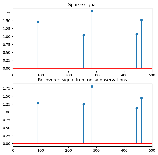
2.1.7. More on the results#
We can plot the sparse signal recovering from the noisy observations to visualize the results.
[12]:
import matplotlib.pyplot as plt
(inx_true,) =  true_params.nonzero()
(inx_est,) =  solver.params.nonzero()

# plot the sparse signal
plt.figure(figsize=(7, 7))
plt.subplot(2, 1, 1)
plt.stem(inx_true, true_params[inx_true], markerfmt='o', basefmt='k-')
plt.plot([0, 500], [0, 0], 'r-', lw=2)
plt.xlim(0, 500)
plt.title("Sparse signal")
#plt.plot(inx_true, true_params[inx_true], drawstyle='steps-post')

# plot the noisy reconstruction
plt.subplot(2, 1, 2)
plt.stem(inx_est, solver.params[inx_est], markerfmt='o', basefmt='k-')
plt.plot([0, 500], [0, 0], 'r-', lw=2)
plt.xlim(0, 500)
plt.title("Recovered signal from noisy observations")
#plt.plot(inx_est, solver.params[inx_est], drawstyle='steps-post')

plt.show()
[ ]: