4.3. Spatial trend filtering

4.3.1. Introduction

Consider a surface data \(Y\in\mathbb{R}^{m\times n}\) over the grid \(\{1, \cdots, m\}\times\{1, \cdots, n\}\). We want to approximate \(Y\) with a piece-wise linear surface \(X\) as follows:

\[\begin{split}X = \begin{bmatrix} x_{11} & x_{12} & x_{13} & \cdots & x_{1n}\\ x_{21} & x_{22} & x_{23} & \cdots & x_{2n}\\ x_{31} & x_{32} & x_{33} & \cdots & x_{3n}\\ \vdots & \vdots & \vdots & \ddots & \vdots\\ x_{m1} & x_{m2} & x_{m3} & \cdots & x_{mn}\\ \end{bmatrix}.\end{split}\]

Note that the matrix \(X\) itself is dense, and the sparsity is imposed on its second order difference of horizontal and verticalsuccessive elements \(x_{i, j-1}-2x_{i,j}+x_{i, j+1}\) and \(x_{i-1, j}-2x_{i,j}+x_{i+1, j}\). To utilize the capacity of sparse optimization of skscope, we need to reparametrize \(X\) with a sparse matrix \(\Theta\).

We introduce another manner to characterizing the piece-wise linear surface \(X\). Consider the following four neighbourhood elements \begin{align*} &x_{i-1, j-1} &x_{i-1, j}\\ &x_{i, j-1} &x_{i, j} \end{align*} and they locate on the same plane if and only if \(x_{i,j}=x_{i-1, j}+x_{i, j-1}-x_{i-1, j-1}\). On the contrary, if there is a jump at the position \((i, j)\), it holds that \(x_{i,j}=x_{i-1, j}+x_{i, j-1}-x_{i-1, j-1}+\theta_{i,j}\) with \(\theta_{i,j}\neq 0\). Thus, we can iteratively represent the dense matrix \(X=(x_{i,j})\) with a sparse matrix \(\Theta=(\theta_{i,j})\). The first row and the first column is represented as

\[x_{11}=\theta_{11}, x_{12}=\theta_{11}+\theta_{12}, \cdots, x_{1n}=\theta_{11}+(n-1)\theta_{12}+(n-2)\theta_{13}\cdots+\theta_{1n}\]

\[x_{11}=\theta_{11}, x_{21}=\theta_{11}+\theta_{21}, \cdots, x_{m1}=\theta_{11}+(m-1)\theta_{21}+(m-2)\theta_{31}\cdots+\theta_{m1}.\]

For other elements, we have for \(i\geq 2, j\geq 2\) that

\[\begin{split}x_{ij}=\sum_{s=1}^i\sum_{t=1}^jc_{st}\theta_{st} \quad\text{ with }\quad c_{st}= \begin{cases} 1 \quad & s=t=1 \\ 1 \quad & s=i, t=j  \\ (i-s)+(j-t) \quad & \text{otherwise} \end{cases} .\end{split}\]

4.3.2. Implementation

Denote \(p=m\times n\), we vectorize the matrices \(X\), \(\Theta\in\mathbb{R}^{m\times n}\) as \(p\)-dimensional vectors \(\mathrm{Vec}(\Theta)\) and \(\mathrm{Vec}(X)\in\mathbb{R}^p\) in a row-wise manner. The following function get_c computes the coefficients \(c_{st}, 1\leq s\leq i, 1\leq t\leq j\) and the function gen_matrix computes the coefficient matrix \(C\) statisfying

\[\mathrm{Vec}(X) = C \mathrm{Vec}(\Theta).\]

import numpy as np
import jax.numpy as jnp
import matplotlib.pyplot as plt
from skscope import ScopeSolver

m, n = 40, 40
p = m * n

def get_c(i, j, s, t):
    if (s > i) or (t > j):
        return 0
    elif (s==0) and (t==0):
        return 1
    elif (s==i) and (t==j):
        return 1
    else:
        return i - s + j - t

# the (k, l) element C(k, l) of the matrix C is gen_matrix(k, l)
def gen_matrix(k, l):
    i = k // n
    j = k % n
    s = l // n
    t = l % n
    return get_c(i, j, s, t)

C = np.zeros((p, p))
for k in range(p):
    for l in range(p):
        C[k, l] = gen_matrix(k, l)

Then, the spatial trend filtering [1] can be formulated as follows

\[\min_{\theta\in\mathbb{R}^p} \|Y-C\theta\|_2^2 \text{ s.t. } \|\theta\|_0\leq \mathrm{sparsity}\]

where \(Y\in\mathbb{R}^{m\times n}\) is a given matrix data, \(C=(c_{st})\in\mathbb{R}^{p\times p}\) is a known coefficient matrix constructed as above, \(\theta\in\mathbb{R}^p\) is the optimized variable and sparsity is a user-defined sparsity parameter.

The following function stf implements the above spatial trend filtering algorithm.

def stf(Y, sparsity):
    m, n = Y.shape
    p = m * n
    y = Y.reshape(-1)

    def custom_objective(params):
        return jnp.mean(jnp.square(y - C @ params))

    solver = ScopeSolver(p, sparsity)
    params = solver.solve(custom_objective)
    Theta_hat = (C @ params).reshape(m, n)
    return Theta_hat

4.3.3. Synthetic data example

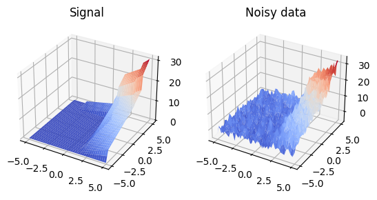
In the following, we generate a piece-wise linear surface \(X\) with the above parameterization such that \(\mathrm{Vec}(X) = C \mathrm{Vec}(\Theta)\) where \(\mathrm{Vec}(\Theta)\) is a \(5\)-sparse vector with all nonzero elements being \(0.2\).

Then, the data \(Y\) is obatined by adding Gaussian noise to \(X\) satisfying \(y_{ij}=x_{ij}+2\mathcal{N}(0, 1), 1\leq i\leq m, 1\leq j\leq n\).

The following figure shows that our parameterization actually has the ability to represent a piece-wise linear surface with a sparse vector.

xx1 = np.linspace(-5, 5, m)
xx2 = np.linspace(-5, 5, n)
X1, X2 = np.meshgrid(xx2, xx2)

theta = np.zeros(p)
pos = np.random.choice(np.arange(p), 5, replace=False)
theta[pos] = 0.2 # np.random.rand(len(pos)) * 5
X = (C @ theta).reshape(m, n)

rng = np.random.default_rng(12345)
noise = rng.standard_normal((m, n)) * 2
Y = X + noise

fig = plt.figure(figsize=(10, 5))

ax1 = fig.add_subplot(131, projection='3d')
ax1.plot_surface(X1, X2, X, cmap='coolwarm')
ax1.set_title('Signal')

ax2 = fig.add_subplot(132, projection='3d')
ax2.plot_surface(X1, X2, Y, cmap='coolwarm')
ax2.set_title('Noisy data')

plt.show()

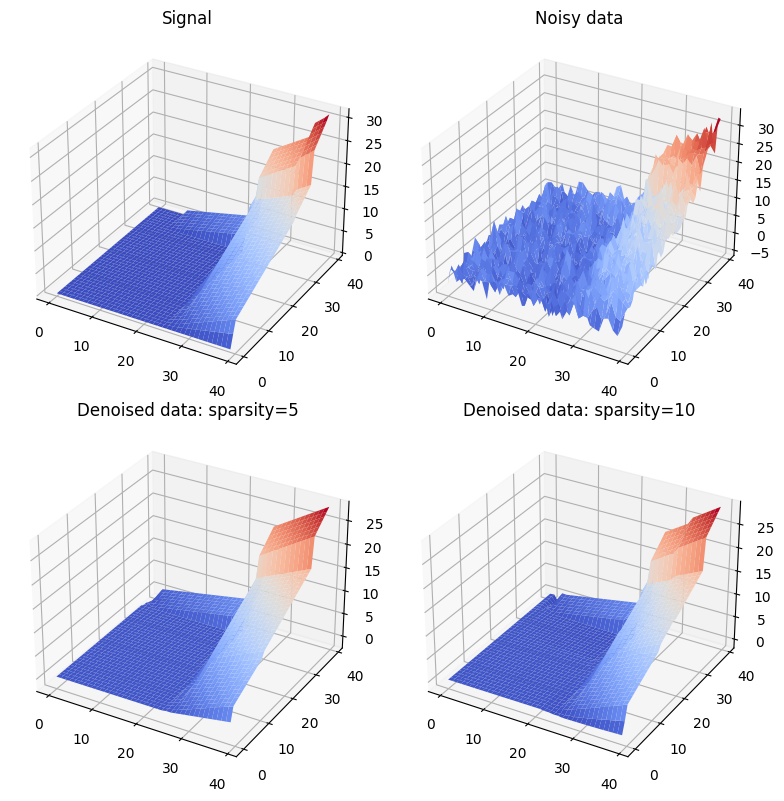
We estimate the true piecewise linear surface \(X\) with two sparsity levels \(5\) and \(10\) and obtain two corresponding estimators X_hat1 and X_hat2.

sparsity1, sparsity2 = 5, 10
X_hat1 = stf(Y, sparsity1)
X_hat2 = stf(Y, sparsity2)

The quality of these two estimators is visualized in the following figure.

Both estimators filter the noisy data \(Y\) and approximate the true piecewise linear surface \(X\) well.

fig = plt.figure(figsize=(8, 8))

xx1 = np.arange(m)
xx2 = np.arange(n)
X1, X2 = np.meshgrid(xx2, xx2)

ax1 = fig.add_subplot(221, projection='3d')
ax1.plot_surface(X1, X2, X, cmap='coolwarm')
ax1.set_title('Signal')

ax2 = fig.add_subplot(222, projection='3d')
ax2.plot_surface(X1, X2, Y, cmap='coolwarm')
ax2.set_title('Noisy data')

ax3 = fig.add_subplot(223, projection='3d')
ax3.plot_surface(X1, X2, X_hat1, cmap='coolwarm')
ax3.set_title('Denoised data: sparsity={}'.format(sparsity1))

ax4 = fig.add_subplot(224, projection='3d')
ax4.plot_surface(X1, X2, X_hat2, cmap='coolwarm')
ax4.set_title('Denoised data: sparsity={}'.format(sparsity2))

plt.tight_layout()
plt.show()

4.3.3.1. Reference

• [1] Kim S J, Koh K, Boyd S, et al. \(\ell_1\) trend filtering[J]. SIAM review, 2009, 51(2): 339-360.