[1]:
%matplotlib inline
2.3. Gamma regression#
2.3.1. Introduction#
Gamma regression is a type of generalized linear model used when the response variable is continuous and strictly positive. It is particularly useful for modeling data such as insurance claim amounts or the lifetime of systems. Gamma regression is widely used in various fields to model positive continuous response variables. Some specific applications include:
Insurance: Estimating the amount of insurance claims based on policyholder characteristics.
Survival Analysis: Modeling the time until an event occurs, such as the lifetime of a machine or system.
Health Economics: Predicting healthcare costs based on patient demographics and medical history.
The Gamma distribution, characterized by a mean parameter (\(\mu\)) and a shape parameter (\(\alpha\)), is defined as follows:
where \(I(\cdot)\) denotes the indicator function. In the context of Gamma regression, the response variable \(y\) is assumed to follow a Gamma distribution:
with the mean parameter \(\mu_i\) modeled as a function of the explanatory variables \(\mathbf{x}_i\):
The Gamma regression model relates the mean of the response variable to the predictors through a link function. The canonical link function for Gamma regression is the inverse link function, which ensures that the mean \(\mu_i\) is always positive. Given \(n\) independent observations of the explanatory variables \(\mathbf{x}\) and the response variable \(y\), the parameter vector \(\boldsymbol{\beta}\) can be estimated by minimizing the negative log-likelihood function under a sparsity constraint:
subject to the constraint \(\|\boldsymbol{\beta}\|_0 \leq s\).
In Gamma regression, the coefficients \(\boldsymbol{\beta}\) have a multiplicative effect on the mean response variable. Specifically, for a unit increase in the predictor \(x_j\), the mean response changes by a factor of \(e^{\beta_j}\), given the inverse link function.
2.3.2. An example#
We would like to use an example to show how the sparse-constrained optimization for gamma regression works in our program.
First, we import some necessary packages and set a seed.
[2]:
import numpy as np
import jax.numpy as jnp
from skscope import ScopeSolver, HTPSolver, GraspSolver
from skscope.numeric_solver import convex_solver_LBFGS
[3]:
np.random.seed(123)
Then, we define a data generator function to provide a way to generate suitable dataset for this task. We consider the model: * \(y \sim \text{Gamma}(\mu, \alpha), \mu = 1/(x^T \beta + \epsilon), \beta \sim U[1, 2], \mu / \alpha\sim U[0.1, 100.1]\) in shape-scale definition.
[4]:
def sample(p, k):
    full = np.arange(p)
    select = sorted(np.random.choice(full, k, replace=False))
    return select

def make_gamma_data(n, p, k, rho=0, corr_type="const", random_state=None):
    np.random.seed(random_state)
    if corr_type == "exp":
        # generate correlation matrix with exponential decay
        R = np.zeros((p, p))
        for i in range(p):
            for j in range(i, p):
                R[i, j] = rho ** abs(i - j)
        R = R + R.T - np.identity(p)
    elif corr_type == "const":
        # generate correlation matrix with constant correlation
        R = np.ones((p, p)) * rho
        for i in range(p):
            R[i, i] = 1
    else:
        raise ValueError(
            "corr_type should be \'const\' or \'exp\'")

    x = np.random.multivariate_normal(mean=np.zeros(p), cov=R, size=(n,))

    nonzero = sample(p, k)
    Tbeta = np.zeros(p)
    sign = np.random.choice([1, -1], k)

    Tbeta[nonzero] = np.random.uniform(1, 2, k) * sign
    # add noise
    eta = x @ Tbeta + np.random.normal(0, 1, n)
    # set coef_0 to make eta>0
    eta = eta + np.abs(np.min(eta)) + 1
    eta = 1 / eta
    # set the shape para of gamma uniformly in [0.1,100.1]
    shape_para = 100 * np.random.uniform(0, 1, 1) + 0.1

    y = np.random.gamma(
        shape=shape_para,
        scale=eta / shape_para,
        size=n)

    return x, y, Tbeta
Next, we use this function to generate a data set containg 500 observations and set only 5 of the 500 variables to have effect on the expectation of the response.
[5]:
n = 500
p = 500
s = 5
x, y, coef_ = make_gamma_data(n=n, p=p, k=s)

print("The predictor variables of the first five samples:",'\n',x[:,:5])
print("The first five noisy observations:", '\n', y[:5])
The predictor variables of the first five samples:
 [[ 1.42438003 -1.67273534  1.68496893 -0.92153038 -0.87169826]
 [-0.4166771   0.07831742  1.60630648  0.78679904  0.33734078]
 [-0.63942892 -1.30434416 -2.37872185  0.28598812 -0.92929139]
 ...
 [-0.2602563   0.09467965 -0.27328825  0.24245864 -0.9253791 ]
 [-0.40261149 -0.44179093 -0.59412831 -0.03653229  3.27678225]
 [-0.81823476 -1.75733214  1.79670648  1.30459205  1.19748667]]
The first five noisy observations:
 [0.10186504 0.07007082 0.07016093 0.10492319 0.06682085]
We augment data to avoid errors in the following codes:
[6]:
X = np.hstack((np.ones((n, 1)), x))
true_params = np.hstack(([0.0], coef_))
Secondly, we define the loss function gamma_loss accorting to 1 that matches the data generating function make_gamma_data.
[7]:
def gamma_loss(params):
    xbeta = jnp.clip(X @ params, -30, 30)
    return jnp.mean(y * xbeta - jnp.log(xbeta))
We note that when computing the gamma loss, \(x_i^T \beta\) may less than 0 and give np.nan or raise error, we should change the initial value of the parameters to make sure that \(x_i^T \beta\) > 0, the following code give an example to deal with this problem.
[8]:
def convex_solver_gamma(
    objective_func,
    value_and_grad,
    params,
    optim_variable_set,
    data,
):
    """
    change the initial value of the parameters to let X @ params > 0
    """
    m = np.min(X @ params)
    if m <= 0.0:
        params[0] -= m
    return convex_solver_LBFGS(objective_func, value_and_grad, params, optim_variable_set, data)
We use skscope to solve the sparse gamma regression problem. After defining the data generation and loss function, we can call ScopeSolver to solve the sparse-constrained optimization problem.
[9]:
solver = ScopeSolver(p+1, s+1, preselect=[0], numeric_solver=convex_solver_gamma)
params = solver.solve(gamma_loss, init_params=np.hstack(([1.0], np.zeros(p))), jit=True)
Now the solver.params contains the coefficients of gamma model with no more than 5 variables.
We can further compare the coefficients estimated by skscope and the real coefficients in two-fold:
The true support set and the estimated support set
The true nonzero parameters and the estimated nonzero parameters
[11]:
true_support_set =  np.nonzero(true_params)[0]
estimated_support_set =  (solver.support_set)[1:]

print("True support set: ", true_support_set)
print("Estimated support set: ", estimated_support_set)
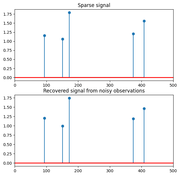
True support set:  [ 94 151 172 374 408]
Estimated support set:  [ 94 151 172 374 408]
[12]:
print("True parameters: ", true_params[true_support_set])
print("Estimated parameters: ", solver.params[estimated_support_set])
True parameters:  [1.16044681 1.06065828 1.78922069 1.20619509 1.55663571]
Estimated parameters:  [1.2021258  0.99600871 1.74258709 1.18841825 1.46535362]
We can find that the support set solved by skscope completely coincides with the support set of the simulation data.
We can plot the sparse signal recovering from the noisy observations to visualize the results.
[13]:
import matplotlib.pyplot as plt

# plot the sparse signal
plt.figure(figsize=(7, 7))
plt.subplot(2, 1, 1)
plt.stem(true_support_set, true_params[true_support_set], markerfmt='o', basefmt='k-')
plt.plot([0, 500], [0, 0], 'r-', lw=2)
plt.xlim(0, 500)
plt.title("Sparse signal")

# plot the noisy reconstruction
plt.subplot(2, 1, 2)
plt.stem(estimated_support_set, solver.params[estimated_support_set], markerfmt='o', basefmt='k-')
plt.plot([0, 500], [0, 0], 'r-', lw=2)
plt.xlim(0, 500)
plt.title("Recovered signal from noisy observations")

plt.show()
2.3.3. References#
[1] Wikipedia, “Gamma distribution”. https://en.wikipedia.org/wiki/Gamma_distribution
[2] Abess docs, “make_glm_data”. https://abess.readthedocs.io/en/latest/Python-package/datasets/glm.html